Lecture 6: Classification using K-Nearest Neighbours

DSCI 100

Worksheets/Tutorials - Week 06


  • Week 6:

    • worksheet_classification1 and tutorial_classification1: Due on Monday, Oct 19

Housekeeping: Midterm Exam

  • Midterm exam is next week, during your own tutorial time slot, starting at the beginning of the tutorial period.
  • Closed book quiz on Canvas: Multiple-choice questions, short answer questions, and fill-in-the-blank questions.
  • Requires Lock Down Browser (LDB)
  • Midterm coverage: Weeks 1 to 6
  • Please see more information under the module “Midterm” in the canvas course page

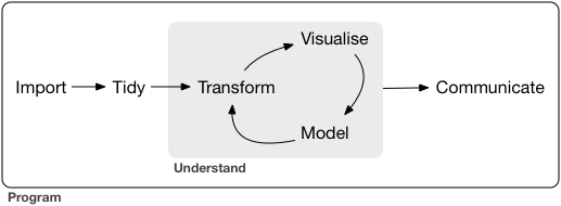
Data Science Workflow

source: R for Data Science by Grolemund & Wickham

Classification

Suppose we have past data of cancer tumour cell diagnosis labelled “benign” and “malignant”. Do you think a new cell with Concavity = 3.3 and Perimeter = 0.2 would be malignant? How did you decide?
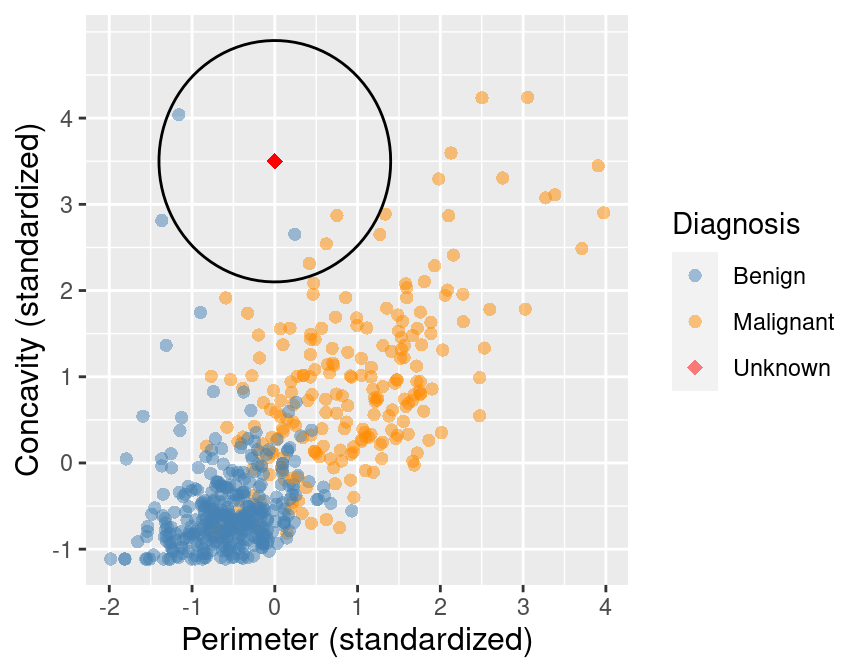
What kind of data analysis question is this?

Descriptive, exploratory, predictive, inferential, causal, or mechanistic?

Notes:

K-nearest Neighbours Classification

Predict the label / class for a new observation using the K closest points from our dataset.

Step 1: Compute the distance between the new observation and each observation in our training set
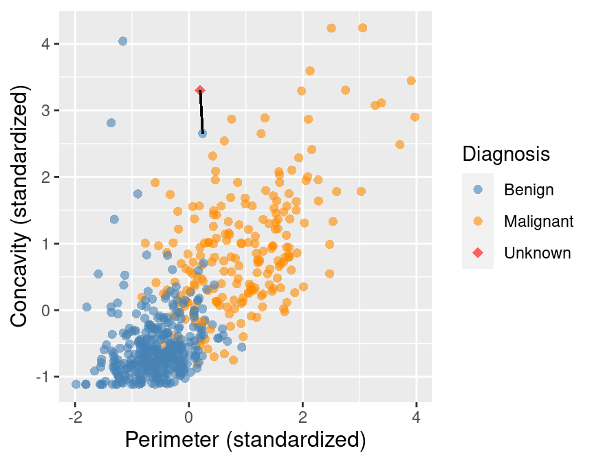
\[ \text{Distance} = \sqrt{ {({\text{new}_x} - {\text{train}_x})^2 + ({\text{new}_y} - {\text{train}_y})^2}} \]

Notes:

K-nearest Neighbours (KNN) Classification

Predict the label / class for a new observation using the K closest points from our dataset.

Step 2: Sort the data in ascending order according to the distances

Step 3: Choose the top K rows as “neighbours”

## # A tibble: 5 x 5
##        ID Perimeter Concavity Class dist_from_new
##     <dbl>     <dbl>     <dbl> <fct>         <dbl>
## 1   86409     0.241      2.65 B             0.881
## 2  887181     0.750      2.87 M             0.980
## 3  899667     0.623      2.54 M             1.14 
## 4  907914     0.417      2.31 M             1.26 
## 5 8710441    -1.16       4.04 B             1.28

K-nearest Neighbours (KNN) Classification

Predict the label / class for a new observation using the K closest points from our dataset.

Step 4: Classify the new observation based on majority vote.
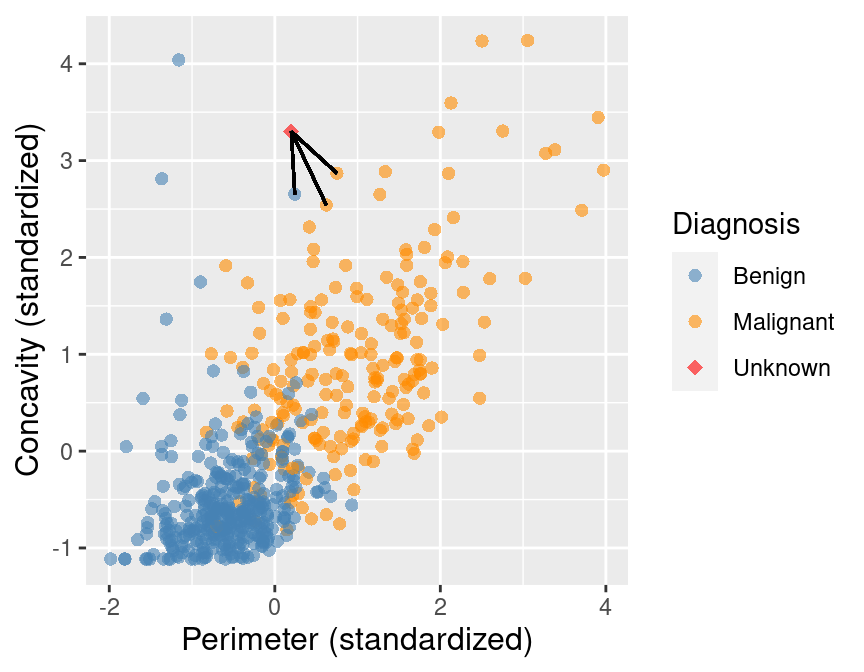
So… what would the predicted class be?

Notes:

Beyond 2 Predictors

For two observations \(u, v\), each with \(m\) variables (columns) labelled \(1, \dots, m\),

\(\text{Distance} = \sqrt{{(u_1-v_1)^2 + (u_2-v_2)^2 + \dots + (u_m - v_m)^2}}\)


Aside from that, it’s the same algorithm!

Standardizing Data

Notes:

Nonstandardized Data

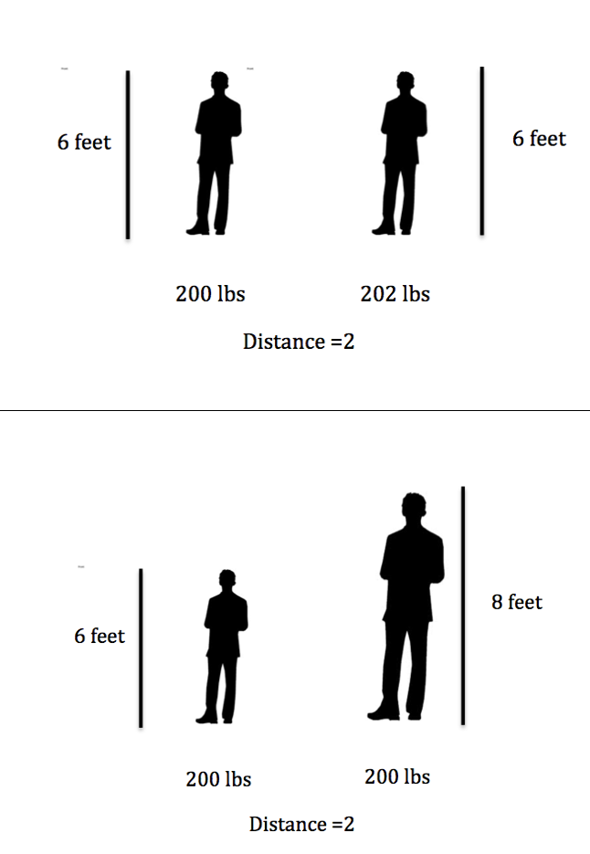
What if one variable is much larger than the other?
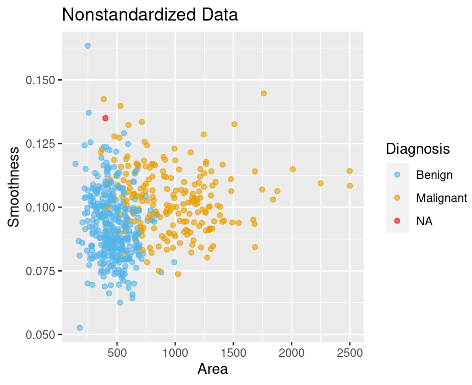
Which observations are closest? What is your initial guess at a classification using K = 3?

Notes:

Nonstandardized Data

What if one variable is much larger than the other?
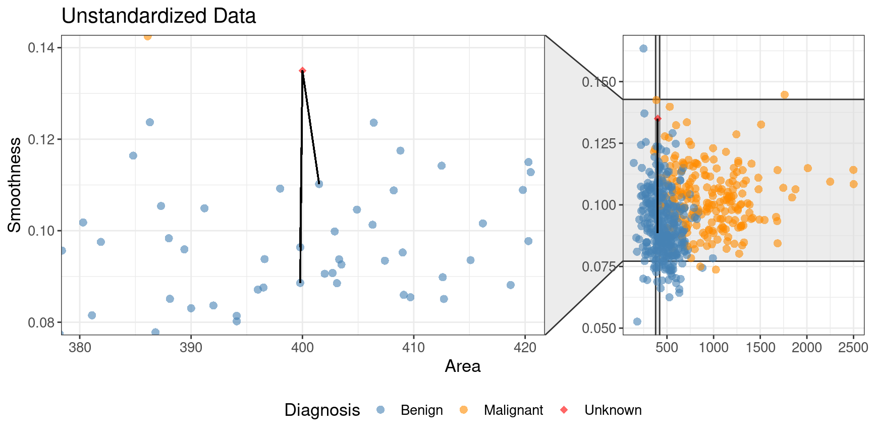
Notes:

Nonstandardized Data vs Standardized Data

What if one variable is much larger than the other?

We need to Standardize: shift and scale so that the average is 0 and the standard deviation (a measure of the spread/variation of the data) is 1.
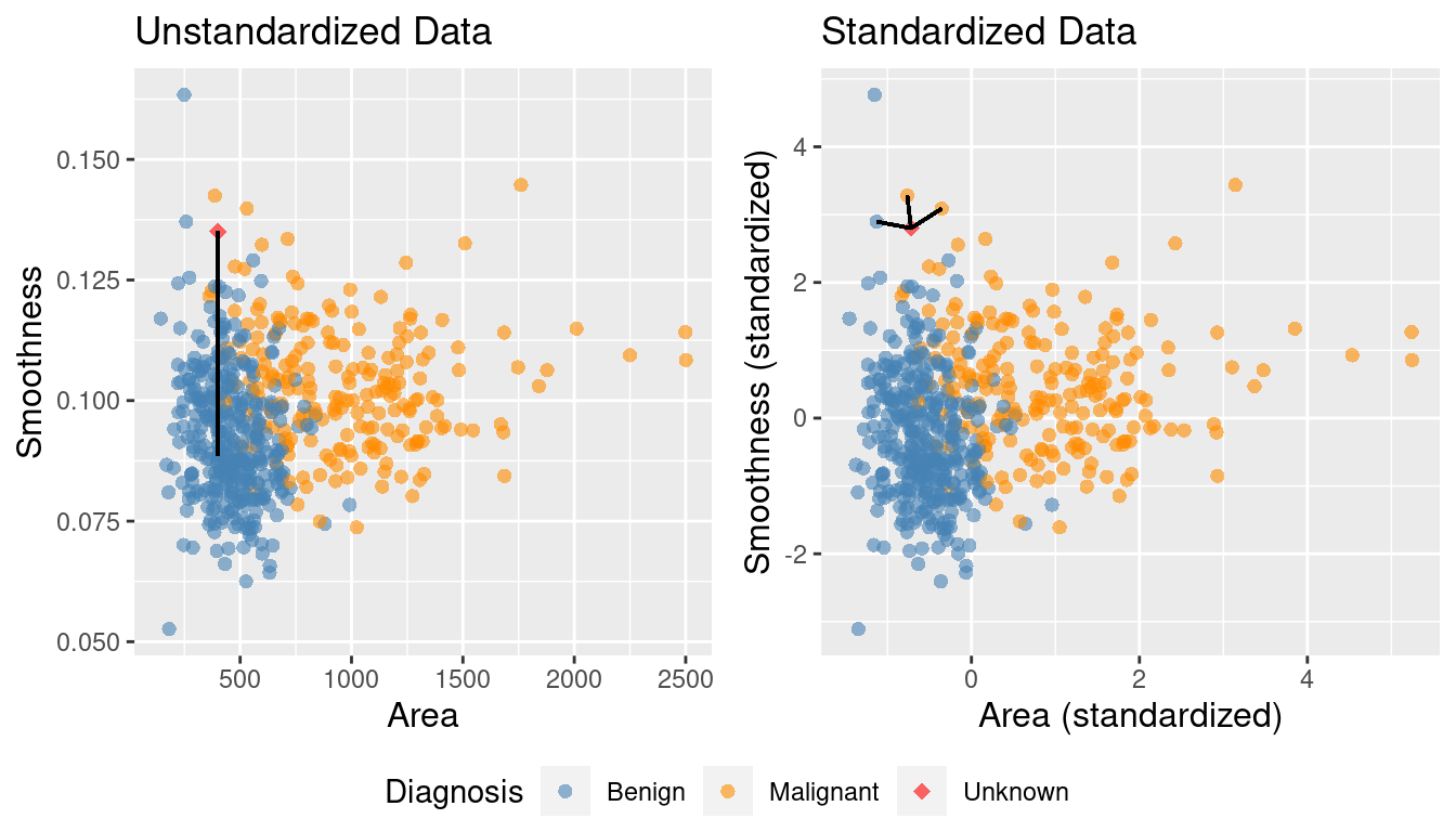
Notes:

Introduction to the tidymodels package in R

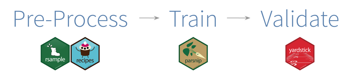
tidymodels is a collection of packages and handles computing distances, standardization, balancing, and prediction for us!
Source: https://www.r-bloggers.com/2019/06/a-gentle-introduction-to-tidymodels/

Introduction to the tidymodels package in R

Step 0a: Load the libraries

Not coding in these slides? You can find clean-wbc.data.csv here

Notes:

Introduction to the tidymodels package in R

Step 0(b): Read in and inspect data we need

Not coding in these slides? You can find clean-wbc.data.csv here

Introduction to the tidymodels package in R

In tidymodels, the recipes package is named after cooking terms.

Step 1: Make a recipe to specify the predictors/response and preprocess the data

  • recipe(): Main function in the formula. Arguments:
-   formula

-    data

You can also prep() and bake() a recipe to see what the preprocessing does! Visit https://recipes.tidymodels.org/reference/index.html to see all the preprocessing steps

Notes:

Let’s standardize our data set:

Notes:

Introduction to the tidymodels package in R

Step 2: Build a model specification (model_spec) to specify the model and training algorithm

  1. model type: kind of model you want to fit

  2. arguments: model parameter values

  3. engine: underlying package the model should come from

  4. mode: type of prediction (some packages can do both classification and regression)

Notes:

Introduction to the tidymodels package in R

Step 3: Put them together in a workflow and then fit it

Notes:

Introduction to the tidymodels package in R

Step 4: Predict a new class label using predict

Notes:

Worksheet Time!

Let’s finish our remaining iClicker questions and begin to work through this week’s worksheet.