DSCI 100 - Introduction to Data Science

Lecture 3 - Wrangling to get tidy data

Credit to Jenny Brian's slides and Garrett Grolemund's tidying example

Housekeeping

• Reminder about worksheets/tutorials:
• do not ever rename, move, or delete your worksheet
  • do not use "Save As..." when you're saving your work
  • use "Save Notebook" or ⌘-s / Ctrl-s instead!
  • at a minimum, if you move/delete/rename worksheets, our autograder won't be able to find them and will give you 0
• You can download your worksheets and tutorials to your computer if you think something has gone terribly wrong.

Reminder

Where are we? Where are we going?

image source: R for Data Science by Grolemund & Wickham

Data Wrangling!

The cartoon illustrations in this slide deck are all created by Allison Horst

• In the real world, when you get data, it's usually very messy
  • inconsistent format (commas, tabs, semicolons, missing data, extra empty lines)
  • split into multiple files (e.g. yearly recorded data over many years)
  • corrupted files, custom formats
• when you read it successfully into R, it will often still be very messy

• you need to make your data "tidy"

What is Tidy Data?

Illustrations from the Openscapes blog Tidy Data for reproducibility, efficiency, and collaboration by Julia Lowndes and Allison Horst"

Examples of Tidy(?) Data

...here is the same data represented in a few different ways. Let's vote on which are tidy!

Tuberculosis data

This data is tidy. True or false?

country	year	rate
Afghanistan	1999	745/19987071
Afghanistan	2000	2666/20595360
Brazil	1999	37737/172006362
Brazil	2000	80488/174504898
China	1999	212258/1272915272
China	2000	213766/1280428583

False.

Tuberculosis data

This data is tidy. True or false?

country	cases (year=1999)	cases (year=2000)	population (year=1999)	population (year=2000)
Afghanistan	745	2666	19987071	20595360
Brazil	37737	80488	172006362	174504898
China	212258	213766	1272915272	1280428583

False. Here we have separate columns for the same variable measured at different years. All population measurements should be contained in a single column, as should all the measurements for cases.

Tuberculosis data

This data is tidy. True or false?

country	1999	2000
Afghanistan	745	2666
Brazil	37737	80488
China	212258	213766

False. Again we have separate columns for the years, and we don't know if the measurement are of population or cases.

Tuberculosis data

This data is tidy. True or false?

country	year	key	value
Afghanistan	1999	cases	745
Afghanistan	1999	population	19987071
Afghanistan	2000	cases	2666
Afghanistan	2000	population	20595360
Brazil	1999	cases	37737
Brazil	1999	population	172006362
Brazil	2000	cases	80488
Brazil	2000	population	174504898
China	1999	cases	212258
China	1999	population	1272915272
China	2000	cases	213766
China	2000	population	1280428583

False. The value column contains measurements of two diffrent variables.

Tuberculosis data

This data is tidy. True or false?

country	year	cases	population
Afghanistan	1999	745	19987071
Afghanistan	2000	2666	20595360
Brazil	1999	37737	172006362
Brazil	2000	80488	174504898
China	1999	212258	1272915272
China	2000	213766	1280428583

True!

• each row corresponds to a single observation,
• each column corresponds to a single variable, and
• each cell (row, column pair) correspond to a single value

Tools for tidying and wrangling data

• tidyverse package functions from:

  • dplyr package (select, filter, mutate, group_by, summarize)

  • tidyr package (pivot_longer, pivot_wider)

  • purrr package (map_dfr)

Demo Time!

library(tidyverse)
library(palmerpenguins)
options(repr.matrix.max.rows = 6)

penguins

Data for 344 penguins. There are 3 different species of penguins in this dataset, collected from 3 islands in the Antarctica.

Select

The select function is used to select a subset of columns (variables) from a dataframe.

# select penguins example

# Recall which column names we have
penguins

# Start with selecting one column
select(penguins, bill_length_mm)

# Select many columns
select(penguins, bill_length_mm,	bill_depth_mm,	flipper_length_mm,	body_mass_g)

# Assign selection
penguins_select <- select(penguins, bill_length_mm,	bill_depth_mm,	flipper_length_mm,	body_mass_g)
penguins_select

# Select all except specfic columns
select(penguins, -island, -species, -sex, -year)

Extra in case students asks about selecting columns more efficiently, e.g. everything that starts with "bill_":

select(penguins, starts_with('bill_'))

These helpers select variables by matching patterns in their names:

• starts_with(): Starts with a prefix.
• ends_with(): Ends with a suffix.
• contains(): Contains a literal string.
• matches(): Matches a regular expression.
• num_range(): Matches a numerical range like x01, x02, x03.

Filter

The filter function is used to choose a subset of rows (observations) in a dataframe.

e.g. filter for only penguins with flippers longer than 190 mm

# penguins filter example

penguins

# One condition
filter(penguins, flipper_length_mm > 190)

# Two conditions
filter(penguins, flipper_length_mm > 190 & species == 'Chinstrap')

Mutate

The mutate function transforms old columns to add new columns.

e.g. convert body mass from grams to pounds

# penguins mutate example

# Recall that 454 g is 1 lbs
mutate(penguins, body_mass_lbs = body_mass_g / 454)

# The above creates a new dataframe, it does not save it to the original `penguins` df
penguins

# We need to assign it to a new variable if we want to save it
penguins_lbs <- mutate(penguins, body_mass_lbs = body_mass_g / 454)

Many operations in the same sequence

When you need type out a long sequence of operations on data, you could either:

1. Save intermediate objects
2. Compose function
3. Use the pipe operator |>

Let's look closer at each one of these

1. Save intermediate objects

penguins_1 <- mutate(penguins, body_mass_lb = body_mass_g/454)
penguins_2 <- filter(penguins_1, flipper_length_mm > 190)
penguins_3 <- select(penguins_2, bill_length_mm, bill_depth_mm, flipper_length_mm, body_mass_lb)
penguins_3

Disadvantages:

• The reader may be tricked into thinking the named penguins_1 and penguins_2 objects are important for some reason, while they are just temporary intermediate computations.
• Further, the reader has to look through and find where penguins_1 and penguins_2 are used in each subsequent line.
• Creating variables that we don't need, could lead to memory issues if they are big and take up a lot of space.

2. Composing functions

penguins_composed <- select(
    filter(
        mutate(
            penguins, body_mass_lb = body_mass_g/454
        ),
        flipper_length_mm > 190
    ),
    bill_length_mm, bill_depth_mm, flipper_length_mm, body_mass_lb
)
penguins_composed

Disadvantage:

• Difficult to read since you the innermost function is exectued first
  • You have to start reading from the middle of the code block (mutate above)

3. Piping

You can also pipe with the |> symbol: passes the output of a function to the 1st argument of another.

penguins_piped <- penguins |>
    mutate(body_mass_lb = body_mass_g/454) |>
    filter(flipper_length_mm > 190) |>
    select(bill_length_mm, bill_depth_mm, flipper_length_mm, body_mass_lb)
penguins_piped

note: if R sees a |> at the end of a line, it keeps reading the next line of code before evaluating!

Advantage:

• Pipes make code much more readable when you need to do a long sequence of operations on data.
• No intermediatery variables created

Nursery rhyme example

Jack and Jill went up the hill
To fetch a pail of water
Jack fell down and broke his crown
And Jill came tumbling after

Intermediate objects

on_hill <- went_up(jack_jill, 'hill')
with_water <- fetch(on_hill, 'water')
fallen <- fell_down(with_water, 'jack')
broken <- broke(fallen, 'jack')
after <- tumble_after(broken, 'jill')

Nursery rhyme example

Jack and Jill went up the hill
To fetch a pail of water
Jack fell down and broke his crown
And Jill came tumbling after

Composing functions

tumble_after(
    broke(
        fell_down(
            fetch(
                went_up(jack_and_jill, "hill"),
                "water"),
            jack),
        "crown"),
    "jill"
)

Nursery rhyme example

Jack and Jill went up the hill
To fetch a pail of water
Jack fell down and broke his crown
And Jill came tumbling after

Pipes

jack_and_jill |>
    went_up("hill") |>
    fetch("water") |>
    fell_down("jack") |>
    broke("crown") |>
    tumble_after("jill")

Credit: https://trestletech.com/wp-content/uploads/2015/07/dplyr.pdf

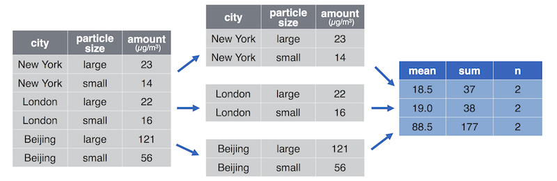
Grouping and summarizing via group_by + summarize

• Grouping is when you split data into groups based on the value of a column.
• Sumarizing is when you combine data into fewer summary values.

For example computing the average particle pollution per city (source https://info201.github.io/dplyr.html):

• Another example, splitting the penguins data into one group per species, and then summarizing the values within each group e.g. reporting the average body_mass per species.
  • To do this we use group_by + summarize to iterate over species, calculating average body mass.

# Recall the data structure
penguins

# Calculate the average body mass for each species

penguins |> 
    group_by(species) |>
    summarize(avg_body_mass = mean(body_mass_g))

Calculate average body mass for each species handling NA's:

penguins |>
    group_by(species) |>
    summarize(avg_body_mass = mean(body_mass_g, na.rm = TRUE))

Count NA's

penguins |>
    summarize(num_nas = sum(is.na(body_mass_g)))

What's going on with those NA's?

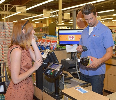
Another big concept this week: iteration

• Iteration is when you need to do something repeatedly (e.g., ringing in and bagging groceries at the till)

• important to reduce duplication of code
• easier to see the intent of your code
• likely have fewer bugs

map_dfr

map_dfr iterates over columns, e.g. to calculate the average for each numeric column in the penguins data

Be careful: There are a lot of map_... functions that you could use (map, map_lgl, map_chr, etc). Usually in this course we'll only use map_dfr, but you should investigate the others yourself!

• map() is a function for applying a function to each element of a list (similar to lapply() )

• map_dfr() returns a data frame

• map() returns a list, map_lgl() a logical vector, map_int() an integer vector, map_dbl() a double vector, and map_chr() a character vector.

• map(YOUR_LIST, YOUR_FUNCTION)

• This data set contains statistics, in arrests per 100,000 residents for assault, murder, and rape in each of the 50 US states in 1973. Also given is the percent of the population living in urban areas.

# Calculate average each numeric column in penguins data set

Returns a df

penguins |>
    select(bill_length_mm:body_mass_g) |>
    map_dfr(mean, na.rm = TRUE)

Returns a list

penguins |>
    select(bill_length_mm:body_mass_g) |>
    map(mean, na.rm = TRUE) |>
#    class()

• Note we can do the same thing with the following but not as efficient, more duplication of code /more prone to errors/less clean:

numeric_penguins  |> 
    summarize(
        mean(bill_length_mm, na.rm = T),
        mean(bill_depth_mm, na.rm = T),
        mean(flipper_length_mm, na.rm = T),
        mean(body_mass_g, na.rm = T),
        mean(year, na.rm = T)
    )

• Vector, Array, List and Data Frame are 4 basic data types defined in R. Knowing the differences between them will help you use R more efficiently.
• Vector: All elements must be of the same type.
• Matrix/array: A matrix is a vector with two additional attributes: the number of rows and the number of columns.
• List can contain elements of different types.
• Dataframe: A data frame is used for storing data tables. It is a list of vectors of equal length.

Go forth and wrangle!

image source: https://media.giphy.com/media/Qgm6tIYrSQqC4/giphy-downsized-large.gif

What did we learn?

Friends with similar tools:

Easier for automation & iteration!

And it makes all other tidy datasets seem more welcoming!

So make friends with tidy data!