Imputation

DSCI 200

Katie Burak, Gabriela V. Cohen Freue

Last modified – 23 February 2026

\[ \DeclareMathOperator*{\argmin}{argmin} \DeclareMathOperator*{\argmax}{argmax} \DeclareMathOperator*{\minimize}{minimize} \DeclareMathOperator*{\maximize}{maximize} \DeclareMathOperator*{\find}{find} \DeclareMathOperator{\st}{subject\,\,to} \newcommand{\E}{E} \newcommand{\Expect}[1]{\E\left[ #1 \right]} \newcommand{\Var}[1]{\mathrm{Var}\left[ #1 \right]} \newcommand{\Cov}[2]{\mathrm{Cov}\left[#1,\ #2\right]} \newcommand{\given}{\ \vert\ } \newcommand{\X}{\mathbf{X}} \newcommand{\x}{\mathbf{x}} \newcommand{\y}{\mathbf{y}} \newcommand{\P}{\mathcal{P}} \newcommand{\R}{\mathbb{R}} \newcommand{\norm}[1]{\left\lVert #1 \right\rVert} \newcommand{\snorm}[1]{\lVert #1 \rVert} \newcommand{\tr}[1]{\mbox{tr}(#1)} \newcommand{\brt}{\widehat{\beta}^R_{s}} \newcommand{\brl}{\widehat{\beta}^R_{\lambda}} \newcommand{\bls}{\widehat{\beta}_{ols}} \newcommand{\blt}{\widehat{\beta}^L_{s}} \newcommand{\bll}{\widehat{\beta}^L_{\lambda}} \newcommand{\U}{\mathbf{U}} \newcommand{\D}{\mathbf{D}} \newcommand{\V}{\mathbf{V}} \]

Attribution

This material is based on content from the following sources:

• The Missing Book
• Flexible Imputation of Missing Data

Learning Objectives

By the end of this lesson, you will be able to:

• Justify and apply strategies for managing the missing data.
• Write a computer script to impute missing values when appropriate
• Write a computer script to evaluate the impact that missing data can have on subsequent analyses through simulation.
• Reflect on the consequences with regards to the conclusions of the chosen method.
• Recognize the importance of utilizing domain knowledge when handling missing data.

Review

Before the midterm we

• introduced the problem of missing data

• learned different ways to diagnose missingness

• defined different missing data mechanisms

• used R functions from naniar package, integrated with tidyverse workflow, to analyzed data

• introduced some imputation methods

Some more details about imputation

• Imputation is not always the solution to missing data

• Imputation can reinforce existing biases.

  • For example, imputing variables like, age, race, gender may introduce biases to the analysis, particularly if missingness is related to social factors.

• In other cases, imputation may mask trends in the data over time.

• The percentage of missing data matters: less than 5% is generally considered safe to impute; 5%–20% is often acceptable but requires careful diagnostics; 20%–40% calls for caution; and more than 40% are typically unreliable.

• When missing data cannot be recovered, it is important to understand why the data are missing and to analyze them accordingly.

Types of imputation

Listwise Deletion

Retain only complete observations

• Simple and widely used

• Unbiased under MCAR

• Biased under MAR in many cases

• Inefficient (larger standard errors due to smaller sample size)

• Discards potentially useful data

Deterministic Methods - I

Imputation using a fix value (e.g., the mean, median, or mode of each variable)

• Replaces missing values using the observed data

• Simple and fast to apply

• Reduces variance

• Introduces bias in relationships among variables

• Ignores imputation uncertainty

library(simputation)
library(naniar)
library(visdat)
library(ggplot2)
library(tidyverse)

set.seed(123)

n <- 100
x1 <- rnorm(n)
x2 <- rnorm(n) + x1
y  <- 2 * x1 + 1.5 * x2 + rnorm(n)

m <- sum(x1 > 0)

set.seed(123)
missing_idx2 <- sample(seq_len(m), size = round(0.5 * m))  # 50% missing
missing_idx1 <- sample(seq_len(m), size = round(0.3 * m))

# introduce MAR
x2[x1 > 0][missing_idx2] <- NA

# introduce MNAR
x1[x1 > 0][head(missing_idx1)] <- NA

simulated_data <- data.frame(x1, x2, y)

simulated_data |>
  nabular() |>
  add_label_shadow() |>
  mutate(across(where(is.numeric), impute_mean)) |> 
  ggplot(aes(x = x1,
             y = x2,
             colour = any_missing)) + geom_point()

Deterministic Methods - II

Statistical Prediction Models

Replaces missing values with predictions from an estimated model (e.g., linear regression) using observed values of other variables

• Preserves relationships between variables

• Assumes relationships that may not be valid

• Ignores imputation uncertainty

simulated_imp_lm <- simulated_data |>
  nabular() |>
  add_label_shadow() |>
  impute_lm(x2 ~ x1 + y)

ggplot(simulated_imp_lm,
       aes(x = x2,
           y = x1,
           colour = any_missing)) +
  geom_point()

Multiple imputation (MI)

Figure from *Flexible Imputation of Missing Data

MI

• Assumes that missing data is either Missing Completely at Random (MCAR) or Missing at Random (MAR).

• Reflects the uncertainty inherent in the missing data by introducing many randomly imputed values.

• Gives unbiased parameter estimates

• Retain the statistical relationships present in the data

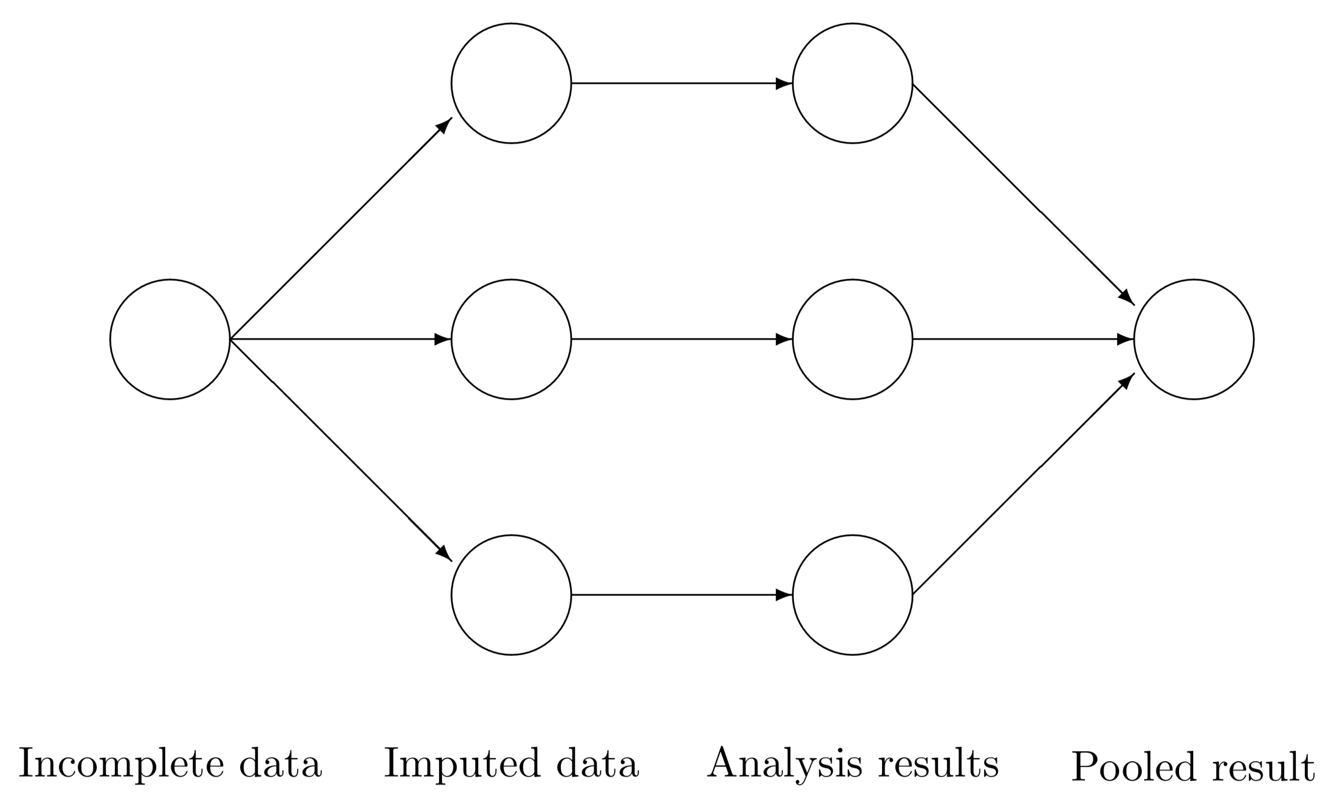
MICE: Multivariate Imputation via Chained Equations

Initialization: Replace missing values with simple initial guesses (e.g., mean or median of observed values).

Imputation: For each variable with missing values, impute it using the other variables as predictors, based on a specified method (e.g., PMM, regression, tree-based methods), including random variation.

Iteration (maxit): Cycle through all variables multiple times to update the imputations.

Multiple Imputations: Repeat to create m complete datasets.

library(mice)
mice_imp <- simulated_data |>
    mice(m = 5, maxit = 10, seed = 123, printFlag =  FALSE)

#one dataset
comp_case <- complete(mice_imp, action = 1)

model_mice1 <- lm(y ~ x1 + x2, data = comp_case)
answer14 <- summary(model_mice1)
answer14

Call:
lm(formula = y ~ x1 + x2, data = comp_case)

Residuals:
     Min       1Q   Median       3Q      Max 
-2.27913 -0.61408 -0.09257  0.51997  2.34976 

Coefficients:
            Estimate Std. Error t value Pr(>|t|)    
(Intercept)  0.05243    0.09369    0.56    0.577    
x1           1.82647    0.13584   13.45   <2e-16 ***
x2           1.44413    0.09194   15.71   <2e-16 ***
---
Signif. codes:  0 '***' 0.001 '**' 0.01 '*' 0.05 '.' 0.1 ' ' 1

Residual standard error: 0.9278 on 97 degrees of freedom
Multiple R-squared:   0.93, Adjusted R-squared:  0.9286 
F-statistic: 644.6 on 2 and 97 DF,  p-value: < 2.2e-16

Visualizing imputation

library(dplyr)
library(mice)

sim_with_flag <- simulated_data |>
  mutate(any_missing = if_any(everything(), is.na))

mice_imp <- mice(sim_with_flag, m = 5, maxit = 10,
                 seed = 123, printFlag = FALSE)

comp_case <- complete(mice_imp, action = 1)

ggplot(comp_case,
       aes(x = x2, y = x1, colour = any_missing)) +
  geom_point()

MICE

Predictive Mean Matching (PMM)

Among many methods implemented in mice, pmm is a popular and default option for imputation of continuous variables

• For each variable with missing values, it fits a regression model using all other variables as predictors

• Computes predicted values for each missing case using the estimated model

• Finds donor candidates among observed cases with matching (close) predicted values

• Randomly selects a donor from the nearest neighbors

• Imputes with the observed value from the chosen donor

Keeps imputed values realistic and within range

Key Takeaways

• Missing data do more than reduce sample size, they can distort who is represented and how variables are related

• Diagnosing why data are missing is essential before choosing how to handle them

• Complete-case analysis is a simple way to handle missingness but is unbiased only under MCAR and often fails otherwise

• MNAR poses the greatest risk of bias when handled incorrectly

• Visualization and diagnostics are critical tools for identifying missingness mechanisms

• naniar integrates missing-data summaries and visualizations into the tidyverse workflow using tidy data principles

• Many imputation methods exist but it is important to understand the risk of imputing!

• Transparent reporting of imputation decisions is essential for reproducibility and ethical integrity.

Check additional functions in the Missing Book