Missing Data

DSCI 200

Katie Burak, Gabriela V. Cohen Freue

Last modified – 04 February 2026

\[ \DeclareMathOperator*{\argmin}{argmin} \DeclareMathOperator*{\argmax}{argmax} \DeclareMathOperator*{\minimize}{minimize} \DeclareMathOperator*{\maximize}{maximize} \DeclareMathOperator*{\find}{find} \DeclareMathOperator{\st}{subject\,\,to} \newcommand{\E}{E} \newcommand{\Expect}[1]{\E\left[ #1 \right]} \newcommand{\Var}[1]{\mathrm{Var}\left[ #1 \right]} \newcommand{\Cov}[2]{\mathrm{Cov}\left[#1,\ #2\right]} \newcommand{\given}{\ \vert\ } \newcommand{\X}{\mathbf{X}} \newcommand{\x}{\mathbf{x}} \newcommand{\y}{\mathbf{y}} \newcommand{\P}{\mathcal{P}} \newcommand{\R}{\mathbb{R}} \newcommand{\norm}[1]{\left\lVert #1 \right\rVert} \newcommand{\snorm}[1]{\lVert #1 \rVert} \newcommand{\tr}[1]{\mbox{tr}(#1)} \newcommand{\brt}{\widehat{\beta}^R_{s}} \newcommand{\brl}{\widehat{\beta}^R_{\lambda}} \newcommand{\bls}{\widehat{\beta}_{ols}} \newcommand{\blt}{\widehat{\beta}^L_{s}} \newcommand{\bll}{\widehat{\beta}^L_{\lambda}} \newcommand{\U}{\mathbf{U}} \newcommand{\D}{\mathbf{D}} \newcommand{\V}{\mathbf{V}} \]

Attribution

This material is based on content from the following sources:

Learning Objectives

Determine potential reasons why data are missing.
Define data missing mechanisms.
Detect instances of missing observations in a data set using a computer script and visualization.
Reflect on the consequences with regards to different ways of handling missing data.
Recognize the importance of utilizing domain knowledge when handling missing data.

The Mystery of Missing Data

Is any data missing?
If so, is there a reason some observations are missing?
How serious is the problem?
What can we do about it?

Examples

Missing data is common in many fields, for example,

Business: missing values may appear in customer surveys, customer profiles, sales records, and inventories.
Healthcare: missing data is common in patient history records, demographics, and clinical variables.
Social Sciences: missing data usually appears in large-scale surveys and administrative records.
Environmental Sciences: missing data frequently occurs in weather station records, air and water quality datasets.

the underlying reasons can differ substantially …

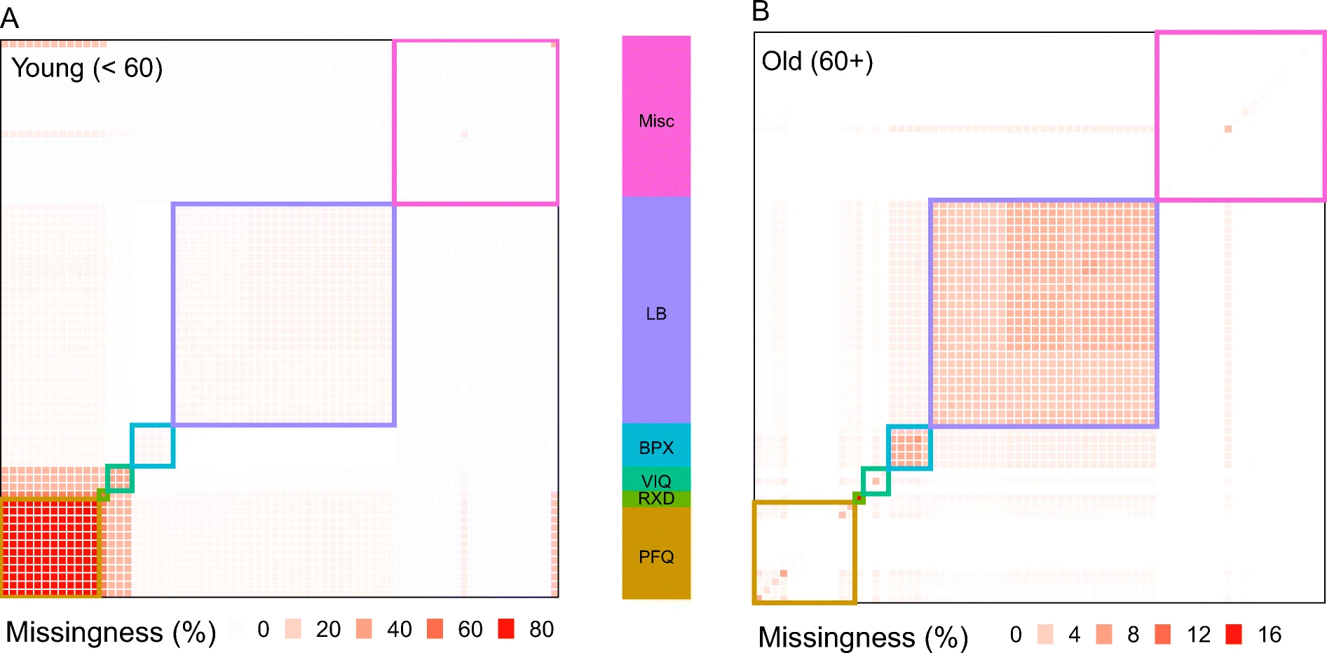
NHANES Data: personal fitness questionnaire (PFQ), number of prescription drugs taken (RXD), vision questionnaire (VIQ), blood pressure measurement (BPX), lab measurements (LB) and miscellaneous (Misc). From Pridham et al., GeroScience 2022.

A Survey of Time Series Analysis Methods and Approaches. SME Water blog.

Not Engaging with Missing Data

Complete-case analysis drops observations with missing values and uses only complete observations, which can result in

substantial bias in estimation
misrepresentation of the population
distort the relation between variables
loss of important information
misleading conclusions

Warning

Many functions in R uses complete data as a default with na.omit = TRUE or na.rm = TRUE

Can Missing Data Tell Us Something?

iClicker 1: exploring missingness

Looking at the COVID-19 map showing percentages of reported cases with missing race/ethnicity data per county. Which statement best describes the missingness?

A. The missing values look randomly scattered

B. The missing values show geographic patterns

C. The missing values are too small to matter

D. There is not enough information to tell

iClicker 2: is missingness informative?

Based on the COVID-19 map, which is the most plausible explanation for why race/ethnicity data are missing in some counties?

A. Random data entry errors

B. Differences in reporting practices or infrastructure

C. The disease affects some races less

D. Pure chance

iClicker 3: consequences of excluding missing data

Suppose we exclude all observations with missing lab measurements (LB) in the NHANES data. What is the most likely consequence?

A. The sample will better represent the population

B. Older adults will be under-represented

C. Estimates of health outcomes will be unbiased

D. Nothing important will change

Why Are Data Missing?

Missing Data Mechanisms

The choice of methods to handle missing data and the validity of subsequent statistical analyses depends strongly on why the data are missing.

Missing Completely at Random (MCAR): as the name suggests, missingness is unrelated to any values, either observed in the dataset or unobserved.
Missing at Random (MAR): missingness is related to observed data, making it easier to explain and handle.
Missing Not at Random (MNAR): missingness is related to unobserved data or the missing values themselves, thus extremely challenging to address.

Key takeaway

Missing data doesn’t just hide information, it can shape who we see and the relationships we infer!

Understanding why data are missing is essential

Mechanism	Depends on	Implications	Example
MCAR	Neither observed nor missing values	Simplest to handle; complete-case analysis reduces sample size but does not add bias	Random sensor failure
MAR	Observed variables only	Complete-case analysis is usually biased; modelling missingness using observed data retains information and attenuates bias	NHANES lab tests missing due to age-based sampling
MNAR	Unobserved variables or the missing values	Missingness must be modeled explicitly; high risk of bias if ignored	Income not reported by high earners

Table adapted from Advanced modeling and data challenges (Vol.3)

Implications of Ignoring the Missingness Mechanism

Understanding why the data are missing is essential to choose an appropriate method to handle it and draw valid conclusions from data:

complete-case analysis can fail when missingness is not truly random
MNAR cases are often associated with sensitive or personal data
ignoring or misshandling MNAR can introduce serious biases, such as underestimating poverty or mischaracterizing population health needs
misdiagnosing missingness can lead to misguided policy or resource allocation decisions

iClicker 4: Identifying MNAR

Which of the following is an example of a context of missing not at random (MNAR)?

A. Income is recorded only for a random subsample of respondents, selected independently of all characteristics.

B. Individuals with lower education levels may omit their education information.

C. Air-quality measurements from ground monitors are missing more often in winter months due to weather-related access issues.

D. Income is missing more often for individuals with temporary or informal employment, which is recorded in the data.

Visualising and Diagnosing Missingness

data("NHANES")
head(NHANES)

# A tibble: 6 × 76
     ID SurveyYr Gender   Age AgeDecade AgeMonths Race1 Race3 Education   
  <int> <fct>    <fct>  <int> <fct>         <int> <fct> <fct> <fct>       
1 51624 2009_10  male      34 " 30-39"        409 White <NA>  High School 
2 51624 2009_10  male      34 " 30-39"        409 White <NA>  High School 
3 51624 2009_10  male      34 " 30-39"        409 White <NA>  High School 
4 51625 2009_10  male       4 " 0-9"           49 Other <NA>  <NA>        
5 51630 2009_10  female    49 " 40-49"        596 White <NA>  Some College
6 51638 2009_10  male       9 " 0-9"          115 White <NA>  <NA>        
# ℹ 67 more variables: MaritalStatus <fct>, HHIncome <fct>, HHIncomeMid <int>,
#   Poverty <dbl>, HomeRooms <int>, HomeOwn <fct>, Work <fct>, Weight <dbl>,
#   Length <dbl>, HeadCirc <dbl>, Height <dbl>, BMI <dbl>,
#   BMICatUnder20yrs <fct>, BMI_WHO <fct>, Pulse <int>, BPSysAve <int>,
#   BPDiaAve <int>, BPSys1 <int>, BPDia1 <int>, BPSys2 <int>, BPDia2 <int>,
#   BPSys3 <int>, BPDia3 <int>, Testosterone <dbl>, DirectChol <dbl>,
#   TotChol <dbl>, UrineVol1 <int>, UrineFlow1 <dbl>, UrineVol2 <int>, …

Even the first lines show that there are some missing values!

str(NHANES)

tibble [10,000 × 76] (S3: tbl_df/tbl/data.frame)
 $ ID              : int [1:10000] 51624 51624 51624 51625 51630 51638 51646 51647 51647 51647 ...
 $ SurveyYr        : Factor w/ 2 levels "2009_10","2011_12": 1 1 1 1 1 1 1 1 1 1 ...
 $ Gender          : Factor w/ 2 levels "female","male": 2 2 2 2 1 2 2 1 1 1 ...
 $ Age             : int [1:10000] 34 34 34 4 49 9 8 45 45 45 ...
 $ AgeDecade       : Factor w/ 8 levels " 0-9"," 10-19",..: 4 4 4 1 5 1 1 5 5 5 ...
 $ AgeMonths       : int [1:10000] 409 409 409 49 596 115 101 541 541 541 ...
 $ Race1           : Factor w/ 5 levels "Black","Hispanic",..: 4 4 4 5 4 4 4 4 4 4 ...
 $ Race3           : Factor w/ 6 levels "Asian","Black",..: NA NA NA NA NA NA NA NA NA NA ...
 $ Education       : Factor w/ 5 levels "8th Grade","9 - 11th Grade",..: 3 3 3 NA 4 NA NA 5 5 5 ...
 $ MaritalStatus   : Factor w/ 6 levels "Divorced","LivePartner",..: 3 3 3 NA 2 NA NA 3 3 3 ...
 $ HHIncome        : Factor w/ 12 levels " 0-4999"," 5000-9999",..: 6 6 6 5 7 11 9 11 11 11 ...
 $ HHIncomeMid     : int [1:10000] 30000 30000 30000 22500 40000 87500 60000 87500 87500 87500 ...
 $ Poverty         : num [1:10000] 1.36 1.36 1.36 1.07 1.91 1.84 2.33 5 5 5 ...
 $ HomeRooms       : int [1:10000] 6 6 6 9 5 6 7 6 6 6 ...
 $ HomeOwn         : Factor w/ 3 levels "Own","Rent","Other": 1 1 1 1 2 2 1 1 1 1 ...
 $ Work            : Factor w/ 3 levels "Looking","NotWorking",..: 2 2 2 NA 2 NA NA 3 3 3 ...
 $ Weight          : num [1:10000] 87.4 87.4 87.4 17 86.7 29.8 35.2 75.7 75.7 75.7 ...
 $ Length          : num [1:10000] NA NA NA NA NA NA NA NA NA NA ...
 $ HeadCirc        : num [1:10000] NA NA NA NA NA NA NA NA NA NA ...
 $ Height          : num [1:10000] 165 165 165 105 168 ...
 $ BMI             : num [1:10000] 32.2 32.2 32.2 15.3 30.6 ...
 $ BMICatUnder20yrs: Factor w/ 4 levels "UnderWeight",..: NA NA NA NA NA NA NA NA NA NA ...
 $ BMI_WHO         : Factor w/ 4 levels "12.0_18.5","18.5_to_24.9",..: 4 4 4 1 4 1 2 3 3 3 ...
 $ Pulse           : int [1:10000] 70 70 70 NA 86 82 72 62 62 62 ...
 $ BPSysAve        : int [1:10000] 113 113 113 NA 112 86 107 118 118 118 ...
 $ BPDiaAve        : int [1:10000] 85 85 85 NA 75 47 37 64 64 64 ...
 $ BPSys1          : int [1:10000] 114 114 114 NA 118 84 114 106 106 106 ...
 $ BPDia1          : int [1:10000] 88 88 88 NA 82 50 46 62 62 62 ...
 $ BPSys2          : int [1:10000] 114 114 114 NA 108 84 108 118 118 118 ...
 $ BPDia2          : int [1:10000] 88 88 88 NA 74 50 36 68 68 68 ...
 $ BPSys3          : int [1:10000] 112 112 112 NA 116 88 106 118 118 118 ...
 $ BPDia3          : int [1:10000] 82 82 82 NA 76 44 38 60 60 60 ...
 $ Testosterone    : num [1:10000] NA NA NA NA NA NA NA NA NA NA ...
 $ DirectChol      : num [1:10000] 1.29 1.29 1.29 NA 1.16 1.34 1.55 2.12 2.12 2.12 ...
 $ TotChol         : num [1:10000] 3.49 3.49 3.49 NA 6.7 4.86 4.09 5.82 5.82 5.82 ...
 $ UrineVol1       : int [1:10000] 352 352 352 NA 77 123 238 106 106 106 ...
 $ UrineFlow1      : num [1:10000] NA NA NA NA 0.094 ...
 $ UrineVol2       : int [1:10000] NA NA NA NA NA NA NA NA NA NA ...
 $ UrineFlow2      : num [1:10000] NA NA NA NA NA NA NA NA NA NA ...
 $ Diabetes        : Factor w/ 2 levels "No","Yes": 1 1 1 1 1 1 1 1 1 1 ...
 $ DiabetesAge     : int [1:10000] NA NA NA NA NA NA NA NA NA NA ...
 $ HealthGen       : Factor w/ 5 levels "Excellent","Vgood",..: 3 3 3 NA 3 NA NA 2 2 2 ...
 $ DaysPhysHlthBad : int [1:10000] 0 0 0 NA 0 NA NA 0 0 0 ...
 $ DaysMentHlthBad : int [1:10000] 15 15 15 NA 10 NA NA 3 3 3 ...
 $ LittleInterest  : Factor w/ 3 levels "None","Several",..: 3 3 3 NA 2 NA NA 1 1 1 ...
 $ Depressed       : Factor w/ 3 levels "None","Several",..: 2 2 2 NA 2 NA NA 1 1 1 ...
 $ nPregnancies    : int [1:10000] NA NA NA NA 2 NA NA 1 1 1 ...
 $ nBabies         : int [1:10000] NA NA NA NA 2 NA NA NA NA NA ...
 $ Age1stBaby      : int [1:10000] NA NA NA NA 27 NA NA NA NA NA ...
 $ SleepHrsNight   : int [1:10000] 4 4 4 NA 8 NA NA 8 8 8 ...
 $ SleepTrouble    : Factor w/ 2 levels "No","Yes": 2 2 2 NA 2 NA NA 1 1 1 ...
 $ PhysActive      : Factor w/ 2 levels "No","Yes": 1 1 1 NA 1 NA NA 2 2 2 ...
 $ PhysActiveDays  : int [1:10000] NA NA NA NA NA NA NA 5 5 5 ...
 $ TVHrsDay        : Factor w/ 7 levels "0_hrs","0_to_1_hr",..: NA NA NA NA NA NA NA NA NA NA ...
 $ CompHrsDay      : Factor w/ 7 levels "0_hrs","0_to_1_hr",..: NA NA NA NA NA NA NA NA NA NA ...
 $ TVHrsDayChild   : int [1:10000] NA NA NA 4 NA 5 1 NA NA NA ...
 $ CompHrsDayChild : int [1:10000] NA NA NA 1 NA 0 6 NA NA NA ...
 $ Alcohol12PlusYr : Factor w/ 2 levels "No","Yes": 2 2 2 NA 2 NA NA 2 2 2 ...
 $ AlcoholDay      : int [1:10000] NA NA NA NA 2 NA NA 3 3 3 ...
 $ AlcoholYear     : int [1:10000] 0 0 0 NA 20 NA NA 52 52 52 ...
 $ SmokeNow        : Factor w/ 2 levels "No","Yes": 1 1 1 NA 2 NA NA NA NA NA ...
 $ Smoke100        : Factor w/ 2 levels "No","Yes": 2 2 2 NA 2 NA NA 1 1 1 ...
 $ Smoke100n       : Factor w/ 2 levels "Non-Smoker","Smoker": 2 2 2 NA 2 NA NA 1 1 1 ...
 $ SmokeAge        : int [1:10000] 18 18 18 NA 38 NA NA NA NA NA ...
 $ Marijuana       : Factor w/ 2 levels "No","Yes": 2 2 2 NA 2 NA NA 2 2 2 ...
 $ AgeFirstMarij   : int [1:10000] 17 17 17 NA 18 NA NA 13 13 13 ...
 $ RegularMarij    : Factor w/ 2 levels "No","Yes": 1 1 1 NA 1 NA NA 1 1 1 ...
 $ AgeRegMarij     : int [1:10000] NA NA NA NA NA NA NA NA NA NA ...
 $ HardDrugs       : Factor w/ 2 levels "No","Yes": 2 2 2 NA 2 NA NA 1 1 1 ...
 $ SexEver         : Factor w/ 2 levels "No","Yes": 2 2 2 NA 2 NA NA 2 2 2 ...
 $ SexAge          : int [1:10000] 16 16 16 NA 12 NA NA 13 13 13 ...
 $ SexNumPartnLife : int [1:10000] 8 8 8 NA 10 NA NA 20 20 20 ...
 $ SexNumPartYear  : int [1:10000] 1 1 1 NA 1 NA NA 0 0 0 ...
 $ SameSex         : Factor w/ 2 levels "No","Yes": 1 1 1 NA 2 NA NA 2 2 2 ...
 $ SexOrientation  : Factor w/ 3 levels "Bisexual","Heterosexual",..: 2 2 2 NA 2 NA NA 1 1 1 ...
 $ PregnantNow     : Factor w/ 3 levels "Yes","No","Unknown": NA NA NA NA NA NA NA NA NA NA ...

The `str()` function gives additional information about the variables, but not about missingness

summary(NHANES)

       ID           SurveyYr       Gender          Age          AgeDecade   
 Min.   :51624   2009_10:5000   female:5020   Min.   : 0.00    40-49 :1398  
 1st Qu.:56904   2011_12:5000   male  :4980   1st Qu.:17.00    0-9   :1391  
 Median :62160                                Median :36.00    10-19 :1374  
 Mean   :61945                                Mean   :36.74    20-29 :1356  
 3rd Qu.:67039                                3rd Qu.:54.00    30-39 :1338  
 Max.   :71915                                Max.   :80.00   (Other):2810  
                                                              NA's   : 333  
   AgeMonths          Race1           Race3               Education   
 Min.   :  0.0   Black   :1197   Asian   : 288   8th Grade     : 451  
 1st Qu.:199.0   Hispanic: 610   Black   : 589   9 - 11th Grade: 888  
 Median :418.0   Mexican :1015   Hispanic: 350   High School   :1517  
 Mean   :420.1   White   :6372   Mexican : 480   Some College  :2267  
 3rd Qu.:624.0   Other   : 806   White   :3135   College Grad  :2098  
 Max.   :959.0                   Other   : 158   NA's          :2779  
 NA's   :5038                    NA's    :5000                        
      MaritalStatus         HHIncome     HHIncomeMid        Poverty     
 Divorced    : 707   more 99999 :2220   Min.   :  2500   Min.   :0.000  
 LivePartner : 560   75000-99999:1084   1st Qu.: 30000   1st Qu.:1.240  
 Married     :3945   25000-34999: 958   Median : 50000   Median :2.700  
 NeverMarried:1380   35000-44999: 863   Mean   : 57206   Mean   :2.802  
 Separated   : 183   45000-54999: 784   3rd Qu.: 87500   3rd Qu.:4.710  
 Widowed     : 456   (Other)    :3280   Max.   :100000   Max.   :5.000  
 NA's        :2769   NA's       : 811   NA's   :811      NA's   :726    
   HomeRooms       HomeOwn             Work          Weight      
 Min.   : 1.000   Own  :6425   Looking   : 311   Min.   :  2.80  
 1st Qu.: 5.000   Rent :3287   NotWorking:2847   1st Qu.: 56.10  
 Median : 6.000   Other: 225   Working   :4613   Median : 72.70  
 Mean   : 6.249   NA's :  63   NA's      :2229   Mean   : 70.98  
 3rd Qu.: 8.000                                  3rd Qu.: 88.90  
 Max.   :13.000                                  Max.   :230.70  
 NA's   :69                                      NA's   :78      
     Length          HeadCirc         Height           BMI       
 Min.   : 47.10   Min.   :34.20   Min.   : 83.6   Min.   :12.88  
 1st Qu.: 75.70   1st Qu.:39.58   1st Qu.:156.8   1st Qu.:21.58  
 Median : 87.00   Median :41.45   Median :166.0   Median :25.98  
 Mean   : 85.02   Mean   :41.18   Mean   :161.9   Mean   :26.66  
 3rd Qu.: 96.10   3rd Qu.:42.92   3rd Qu.:174.5   3rd Qu.:30.89  
 Max.   :112.20   Max.   :45.40   Max.   :200.4   Max.   :81.25  
 NA's   :9457     NA's   :9912    NA's   :353     NA's   :366    
    BMICatUnder20yrs         BMI_WHO         Pulse           BPSysAve    
 UnderWeight:  55    12.0_18.5   :1277   Min.   : 40.00   Min.   : 76.0  
 NormWeight : 805    18.5_to_24.9:2911   1st Qu.: 64.00   1st Qu.:106.0  
 OverWeight : 193    25.0_to_29.9:2664   Median : 72.00   Median :116.0  
 Obese      : 221    30.0_plus   :2751   Mean   : 73.56   Mean   :118.2  
 NA's       :8726    NA's        : 397   3rd Qu.: 82.00   3rd Qu.:127.0  
                                         Max.   :136.00   Max.   :226.0  
                                         NA's   :1437     NA's   :1449   
    BPDiaAve          BPSys1          BPDia1           BPSys2     
 Min.   :  0.00   Min.   : 72.0   Min.   :  0.00   Min.   : 76.0  
 1st Qu.: 61.00   1st Qu.:106.0   1st Qu.: 62.00   1st Qu.:106.0  
 Median : 69.00   Median :116.0   Median : 70.00   Median :116.0  
 Mean   : 67.48   Mean   :119.1   Mean   : 68.28   Mean   :118.5  
 3rd Qu.: 76.00   3rd Qu.:128.0   3rd Qu.: 76.00   3rd Qu.:128.0  
 Max.   :116.00   Max.   :232.0   Max.   :118.00   Max.   :226.0  
 NA's   :1449     NA's   :1763    NA's   :1763     NA's   :1647   
     BPDia2           BPSys3          BPDia3       Testosterone    
 Min.   :  0.00   Min.   : 76.0   Min.   :  0.0   Min.   :   0.25  
 1st Qu.: 60.00   1st Qu.:106.0   1st Qu.: 60.0   1st Qu.:  17.70  
 Median : 68.00   Median :116.0   Median : 68.0   Median :  43.82  
 Mean   : 67.66   Mean   :117.9   Mean   : 67.3   Mean   : 197.90  
 3rd Qu.: 76.00   3rd Qu.:126.0   3rd Qu.: 76.0   3rd Qu.: 362.41  
 Max.   :118.00   Max.   :226.0   Max.   :116.0   Max.   :1795.60  
 NA's   :1647     NA's   :1635    NA's   :1635    NA's   :5874     
   DirectChol       TotChol         UrineVol1       UrineFlow1     
 Min.   :0.390   Min.   : 1.530   Min.   :  0.0   Min.   : 0.0000  
 1st Qu.:1.090   1st Qu.: 4.110   1st Qu.: 50.0   1st Qu.: 0.4030  
 Median :1.290   Median : 4.780   Median : 94.0   Median : 0.6990  
 Mean   :1.365   Mean   : 4.879   Mean   :118.5   Mean   : 0.9793  
 3rd Qu.:1.580   3rd Qu.: 5.530   3rd Qu.:164.0   3rd Qu.: 1.2210  
 Max.   :4.030   Max.   :13.650   Max.   :510.0   Max.   :17.1670  
 NA's   :1526    NA's   :1526     NA's   :987     NA's   :1603     
   UrineVol2       UrineFlow2     Diabetes     DiabetesAge        HealthGen   
 Min.   :  0.0   Min.   : 0.000   No  :9098   Min.   : 1.00   Excellent: 878  
 1st Qu.: 52.0   1st Qu.: 0.475   Yes : 760   1st Qu.:40.00   Vgood    :2508  
 Median : 95.0   Median : 0.760   NA's: 142   Median :50.00   Good     :2956  
 Mean   :119.7   Mean   : 1.149               Mean   :48.42   Fair     :1010  
 3rd Qu.:171.8   3rd Qu.: 1.513               3rd Qu.:58.00   Poor     : 187  
 Max.   :409.0   Max.   :13.692               Max.   :80.00   NA's     :2461  
 NA's   :8522    NA's   :8524                 NA's   :9371                    
 DaysPhysHlthBad  DaysMentHlthBad  LittleInterest   Depressed   
 Min.   : 0.000   Min.   : 0.000   None   :5103   None   :5246  
 1st Qu.: 0.000   1st Qu.: 0.000   Several:1130   Several:1009  
 Median : 0.000   Median : 0.000   Most   : 434   Most   : 418  
 Mean   : 3.335   Mean   : 4.126   NA's   :3333   NA's   :3327  
 3rd Qu.: 3.000   3rd Qu.: 4.000                                
 Max.   :30.000   Max.   :30.000                                
 NA's   :2468     NA's   :2466                                  
  nPregnancies       nBabies         Age1stBaby    SleepHrsNight   
 Min.   : 1.000   Min.   : 0.000   Min.   :14.00   Min.   : 2.000  
 1st Qu.: 2.000   1st Qu.: 2.000   1st Qu.:19.00   1st Qu.: 6.000  
 Median : 3.000   Median : 2.000   Median :22.00   Median : 7.000  
 Mean   : 3.027   Mean   : 2.457   Mean   :22.65   Mean   : 6.928  
 3rd Qu.: 4.000   3rd Qu.: 3.000   3rd Qu.:26.00   3rd Qu.: 8.000  
 Max.   :32.000   Max.   :12.000   Max.   :39.00   Max.   :12.000  
 NA's   :7396     NA's   :7584     NA's   :8116    NA's   :2245    
 SleepTrouble PhysActive  PhysActiveDays       TVHrsDay        CompHrsDay  
 No  :5799    No  :3677   Min.   :1.000   2_hr     :1275   0_to_1_hr:1409  
 Yes :1973    Yes :4649   1st Qu.:2.000   1_hr     : 884   0_hrs    :1073  
 NA's:2228    NA's:1674   Median :3.000   3_hr     : 836   1_hr     :1030  
                          Mean   :3.744   0_to_1_hr: 638   2_hr     : 589  
                          3rd Qu.:5.000   More_4_hr: 615   3_hr     : 347  
                          Max.   :7.000   (Other)  : 611   (Other)  : 415  
                          NA's   :5337    NA's     :5141   NA's     :5137  
 TVHrsDayChild   CompHrsDayChild Alcohol12PlusYr   AlcoholDay    
 Min.   :0.000   Min.   :0.000   No  :1368       Min.   : 1.000  
 1st Qu.:1.000   1st Qu.:0.000   Yes :5212       1st Qu.: 1.000  
 Median :2.000   Median :1.000   NA's:3420       Median : 2.000  
 Mean   :1.939   Mean   :2.197                   Mean   : 2.914  
 3rd Qu.:3.000   3rd Qu.:6.000                   3rd Qu.: 3.000  
 Max.   :6.000   Max.   :6.000                   Max.   :82.000  
 NA's   :9347    NA's   :9347                    NA's   :5086    
  AlcoholYear    SmokeNow    Smoke100         Smoke100n       SmokeAge    
 Min.   :  0.0   No  :1745   No  :4024   Non-Smoker:4024   Min.   : 6.00  
 1st Qu.:  3.0   Yes :1466   Yes :3211   Smoker    :3211   1st Qu.:15.00  
 Median : 24.0   NA's:6789   NA's:2765   NA's      :2765   Median :17.00  
 Mean   : 75.1                                             Mean   :17.83  
 3rd Qu.:104.0                                             3rd Qu.:19.00  
 Max.   :364.0                                             Max.   :72.00  
 NA's   :4078                                              NA's   :6920   
 Marijuana   AgeFirstMarij   RegularMarij  AgeRegMarij    HardDrugs  
 No  :2049   Min.   : 1.00   No  :3575    Min.   : 5.00   No  :4700  
 Yes :2892   1st Qu.:15.00   Yes :1366    1st Qu.:15.00   Yes :1065  
 NA's:5059   Median :16.00   NA's:5059    Median :17.00   NA's:4235  
             Mean   :17.02                Mean   :17.69              
             3rd Qu.:19.00                3rd Qu.:19.00              
             Max.   :48.00                Max.   :52.00              
             NA's   :7109                 NA's   :8634               
 SexEver         SexAge      SexNumPartnLife   SexNumPartYear   SameSex    
 No  : 223   Min.   : 9.00   Min.   :   0.00   Min.   : 0.000   No  :5353  
 Yes :5544   1st Qu.:15.00   1st Qu.:   2.00   1st Qu.: 1.000   Yes : 415  
 NA's:4233   Median :17.00   Median :   5.00   Median : 1.000   NA's:4232  
             Mean   :17.43   Mean   :  15.09   Mean   : 1.342              
             3rd Qu.:19.00   3rd Qu.:  12.00   3rd Qu.: 1.000              
             Max.   :50.00   Max.   :2000.00   Max.   :69.000              
             NA's   :4460    NA's   :4275      NA's   :5072                
      SexOrientation  PregnantNow  
 Bisexual    : 119   Yes    :  72  
 Heterosexual:4638   No     :1573  
 Homosexual  :  85   Unknown:  51  
 NA's        :5158   NA's   :8304

The `summary()` function gives only a count of missing values per variable, but not how missingness relates across variables

Plots can be especially useful for visualizing patterns and relationships in missingness

Variable-wise summaries (gg_miss_var): show missingness in each variable
- helping identify which variables are most affected
Heatmaps (vis_miss): show where values are missing across observations and variables
- useful for spotting structure, clustering, or blocks of missingness
UpSet plots (gg_miss_upset): show which combinations of variables tend to be missing together
- revealing joint or structural missingness patterns.
Missingness vs Covariates (gg_miss_fct, geom_miss_point): show how missingness relates to observed variables
- helping assess whether missingness may depend on observed data (MAR)

vis_dat(NHANES)+
  theme(axis.text.x = element_text(angle = 90, vjust = 0.5, size = 6), legend.position = "bottom")

vis_dat() functions is useful to visualize the structure of the data and missingness

#Variable-wise summary
NHANES %>%
  gg_miss_var()+
  theme(axis.text.y = element_text(size = 4))

the dataset has too many variables for these visualizations
- variable names become difficult to read
the plot is still useful to have an overall idea of the amount of missingness per variables

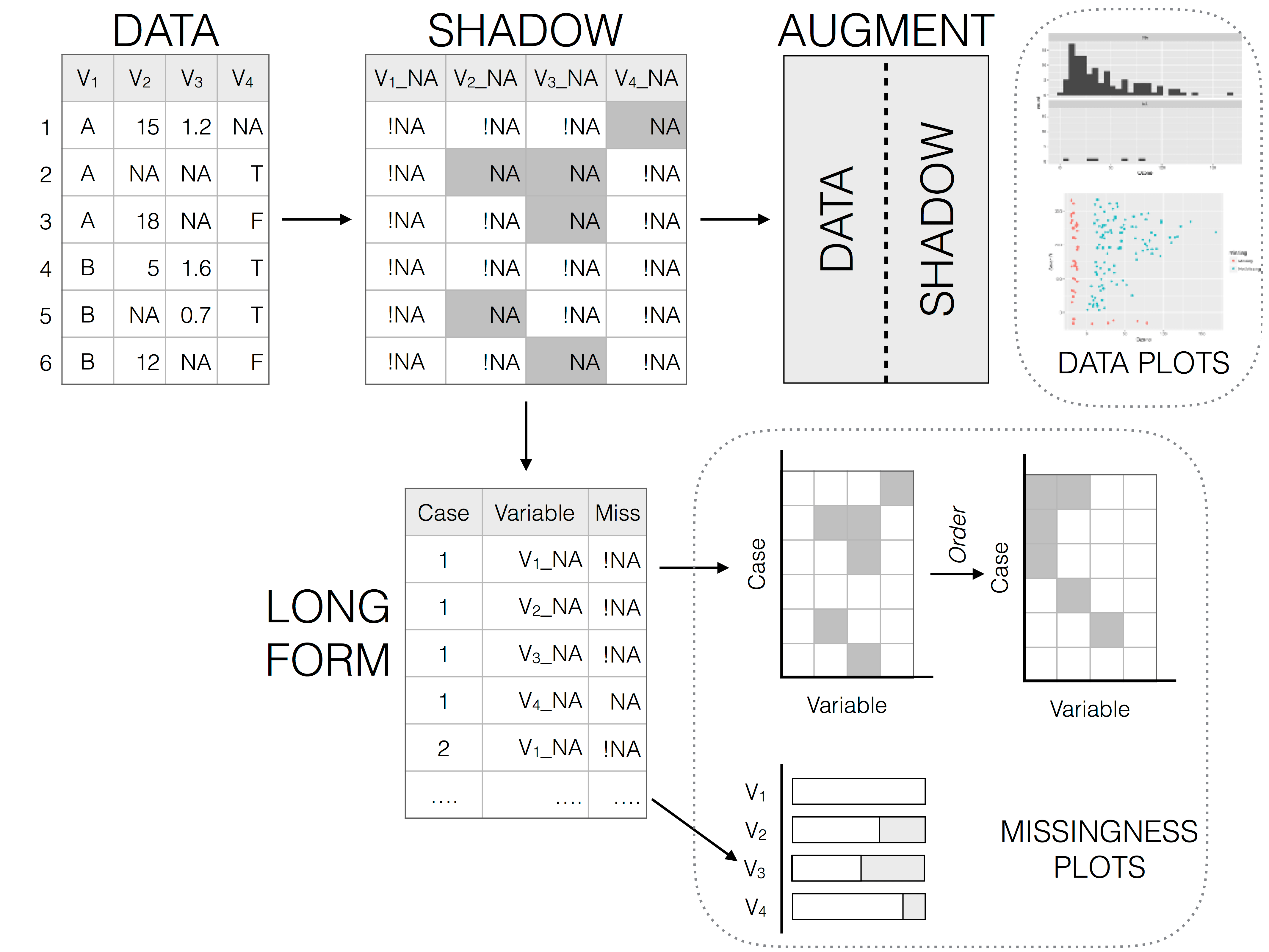
naniar creates a “shadow” matrix to store the missing data structure in a tidy format
- useful to create visualizations and wrangle data

#Heatmap
vis_miss(NHANES) +
  theme(axis.text.x = element_text(angle = 90, vjust = 0.5, size = 6))

Look at subset of variables to understand missingness patterns

Some variables are mutually exclusive by design

Some variables are jointly missing, can be because of the design of the study too

When blood pressure is missing, what else is missing?

Diagnosing the Missingness Mechanism for BP

BP missingness appears to be part of a larger missingness module
- some participants are missing an entire exam/measurements
- likely not MCAR
- can be MAR if the chance of being in that “missing block” is explainable by observed variables (e.g., age group, survey year, type of examination)
- can be MNAR if missingness depends on unobserved health status
- we can’t diagnose MNAR from this plot alone

`SurveyYr` doesn’t seem to explain the block missingness observed

Some variables are jointly missing but differing per age groups, suggesting MAR

nhanes_shadow <- bind_shadow(NHANES)
ggplot(nhanes_shadow,
       aes(x = Age,
           colour = BPSysAve_NA)) + 
  geom_density()

Missingness in blood pressure is mostly related to age, suggesting MAR

#UpSet plot
gg_miss_upset(bp_block,nsets=6)

NHANES %>%
  select(BMI, Age, Weight, Height, Pulse, BPSysAve, BPDiaAve) %>%
  gg_miss_upset(nsets=6)

ggplot(
  data = NHANES,
  mapping = aes(x = Weight, y = BMI)) +     
  geom_miss_point() +
  theme(legend.position = "bottom")

Missing values of one variable in relation to the non-missing values of the other (red dots)

Summaries of missingness

per variable

NHANES %>%
  select(AgeDecade, BMI, Weight, Height, Pulse,   starts_with("BP")) %>% 
  miss_var_summary()

# A tibble: 13 × 3
   variable  n_miss pct_miss
   <chr>      <int>    <num>
 1 BPSys1      1763    17.6 
 2 BPDia1      1763    17.6 
 3 BPSys2      1647    16.5 
 4 BPDia2      1647    16.5 
 5 BPSys3      1635    16.4 
 6 BPDia3      1635    16.4 
 7 BPSysAve    1449    14.5 
 8 BPDiaAve    1449    14.5 
 9 Pulse       1437    14.4 
10 BMI          366     3.66
11 Height       353     3.53
12 AgeDecade    333     3.33
13 Weight        78     0.78

per cases (rows)

# Percent of rows with at least one missing value
pct_miss_case(NHANES)

[1] 100

Key Takeaways

Missing data do more than reduce sample size, they can distort who is represented and how variables are related
Diagnosing why data are missing is essential before choosing how to handle them
Complete-case analysis is a simple way to handle missingness but is unbiased only under MCAR and often fails otherwise
MNAR poses the greatest risk of bias when handled incorrectly
Visualization and diagnostics are critical tools for identifying missingness mechanisms
naniar integrates missing-data summaries and visualizations into the tidyverse workflow using tidy data principles

Missing Data

Attribution

Learning Objectives

The Mystery of Missing Data

Examples

the underlying reasons can differ substantially …

Not Engaging with Missing Data

Can Missing Data Tell Us Something?

iClicker 1: exploring missingness

iClicker 2: is missingness informative?

iClicker 3: consequences of excluding missing data

Why Are Data Missing?

Missing Data Mechanisms

Understanding why data are missing is essential

Implications of Ignoring the Missingness Mechanism

iClicker 4: Identifying MNAR

Visualising and Diagnosing Missingness

Even the first lines show that there are some missing values!

The str() function gives additional information about the variables, but not about missingness

The summary() function gives only a count of missing values per variable, but not how missingness relates across variables

When blood pressure is missing, what else is missing?

Diagnosing the Missingness Mechanism for BP

SurveyYr doesn’t seem to explain the block missingness observed

Some variables are jointly missing but differing per age groups, suggesting MAR

Summaries of missingness

per variable

per cases (rows)

Key Takeaways

Check additional functions in the Missing Book

The `str()` function gives additional information about the variables, but not about missingness

The `summary()` function gives only a count of missing values per variable, but not how missingness relates across variables

`SurveyYr` doesn’t seem to explain the block missingness observed