Outliers I

DSCI 200

Katie Burak, Gabriela V. Cohen Freue

Last modified – 09 March 2026

\[ \DeclareMathOperator*{\argmin}{argmin} \DeclareMathOperator*{\argmax}{argmax} \DeclareMathOperator*{\minimize}{minimize} \DeclareMathOperator*{\maximize}{maximize} \DeclareMathOperator*{\find}{find} \DeclareMathOperator{\st}{subject\,\,to} \newcommand{\E}{E} \newcommand{\Expect}[1]{\E\left[ #1 \right]} \newcommand{\Var}[1]{\mathrm{Var}\left[ #1 \right]} \newcommand{\Cov}[2]{\mathrm{Cov}\left[#1,\ #2\right]} \newcommand{\given}{\ \vert\ } \newcommand{\X}{\mathbf{X}} \newcommand{\x}{\mathbf{x}} \newcommand{\y}{\mathbf{y}} \newcommand{\P}{\mathcal{P}} \newcommand{\R}{\mathbb{R}} \newcommand{\norm}[1]{\left\lVert #1 \right\rVert} \newcommand{\snorm}[1]{\lVert #1 \rVert} \newcommand{\tr}[1]{\mbox{tr}(#1)} \newcommand{\brt}{\widehat{\beta}^R_{s}} \newcommand{\brl}{\widehat{\beta}^R_{\lambda}} \newcommand{\bls}{\widehat{\beta}_{ols}} \newcommand{\blt}{\widehat{\beta}^L_{s}} \newcommand{\bll}{\widehat{\beta}^L_{\lambda}} \newcommand{\U}{\mathbf{U}} \newcommand{\D}{\mathbf{D}} \newcommand{\V}{\mathbf{V}} \]

Attribution

• Some examples and references are from Challenges of cellwise outliers, by Raymaekers and Rousseeuw

• Robust Statistics, by Maronna, Martin, Yohai, Salibian-Barrera

In memory of my mentor and friend

Professor Ruben Zamar (1949-2023)

who contributed greatly to Robust Statistics and beyond …

Learning Objectives

By the end of this lesson, you will be able to:

• Determine potential reasons why data contain outliers.
• Compare outliers with extreme values generated from heavy-tailed distributions.
• Recognize different types of outliers in a data set (e.g., casewise versus cellwise outliers).
• Use different methods to detect outliers in a data set and understand differences in the results.
• Justify and apply strategies for managing outliers in the data, including transformations and data imputation.
• Write a computer script to evaluate the impact that outliers can have on subsequent analyses through simulation.
• Reflect on the consequences with regards to the conclusions of the chosen method.
• Recognize the importance of utilizing domain knowledge when handling outliers.

What is an outlier?

Outliers

Definition: Outlier

An outlier is an observation that deviates from the bulk of the data, an atypical observation.

Outliers may arise from:

• errors when collecting or processing data

• values generated from a different distribution

• rare cases which may carry valuable information

As with missing values, outliers require careful diagnosis and appropriate handling before analysis.

Casewise vs Cellwise

Casewise

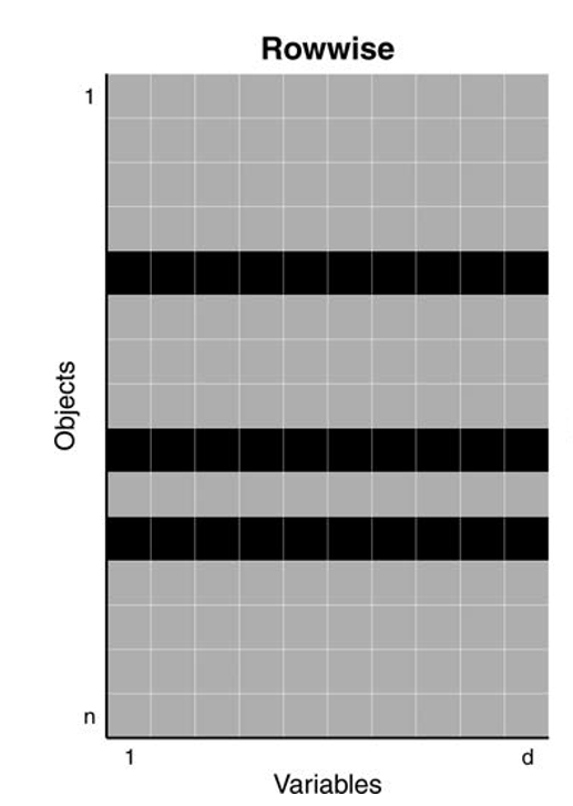
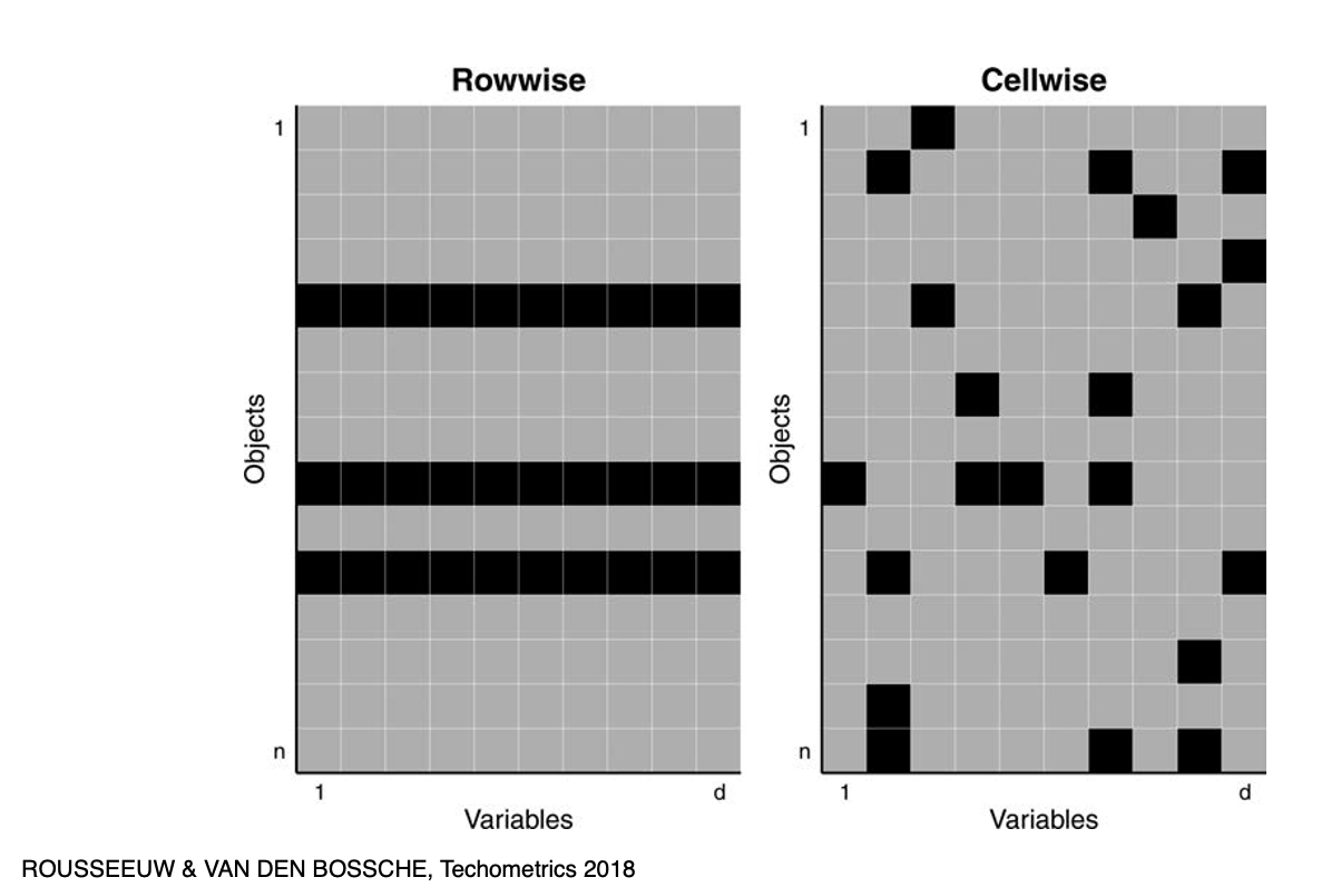
In the 1960s Tukey and Huber introduced the casewise (aka rowwise) contamination model

• Treats entire rows as contaminated and coming from a different distribution, even if only values of some variables are unusual

• Assumes that less than 50% of the cases (objects) are contaminated

Cellwise

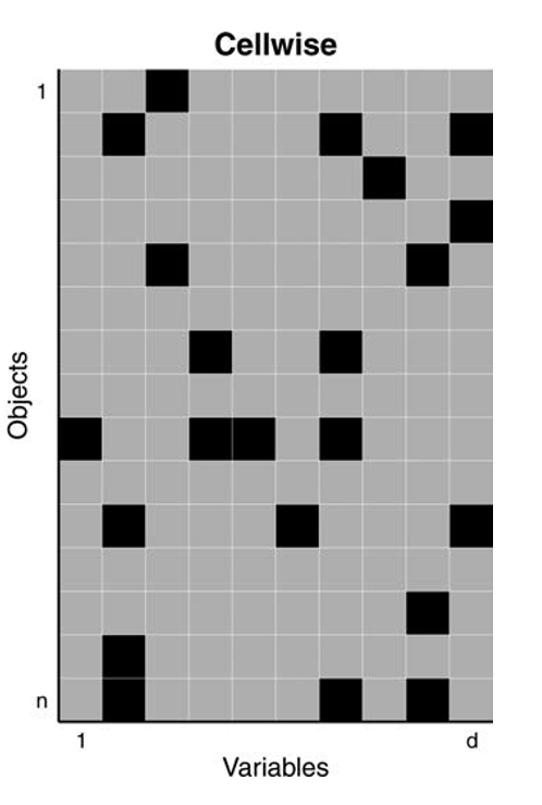
In 2009, Alqallaf, Van Aelst, Yohai and Zamar introduced the cellwise contamination model

• Only individual cells are contaminated, with values coming from a different distribution

• Any case (row) may contain some contaminated cells

• More realistic for high-dimensional data

Glass data

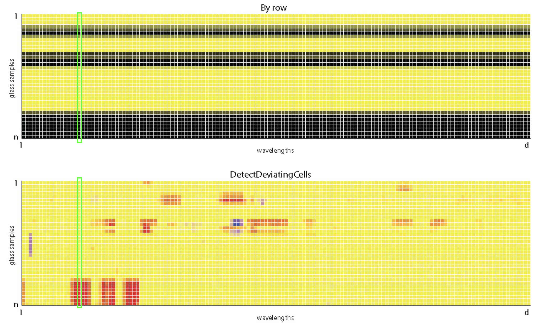
Data: n = 180 archeological glass spectra with d = 750 wavelengths (Detecting Deviating Data Cells, Rousseeuw & Van Den Bossche, Technometrics 2018)

Univariate estimators

Before analyzing multivariate datasets, we first need to learn how to identify and handle outlying values in a single variable.

Let’s look at the values of the wavelength V169 in this data

Robust estimators

• Classical estimators can be highly distorted by outliers

• Robust estimators are needed to capture the bulk of the data

• Robust estimators are also needed to flag outliers

Statistic	Estimate
Mean	5260.72
Median	4629
SD	1413.69
MAD	470.73

The mean and SD are very sensitive to the outliers in the data

Mean (\(\bar{X}\)) vs Median (\(\tilde{X}\))

If the median is less affected by extreme values, why not using it as a default?

• if the data contain outliers, the median is more resistant

• but if the data does not contain outliers, it is less efficient (larger standard error!)

If data is Normally distributed:

\[SE(\bar{X}) = \frac{\sigma}{\sqrt{n}}\]

\[SE(\tilde{X})= \sqrt{\frac{\pi}{2}}\frac{\sigma}{\sqrt{n}}\]

Let’s examine these two points by simulation!

Simulation design

Clean data

• Generate a sample of size 100 from a Normal distribution with mean 0 and standard deviation 1

• Compute the mean and the median

• Repeat 10000 times

• Summarize their sampling distributions

set.seed(200)

sim_stats <- replicate(10000, {
  x <- rnorm(100)
  c(mean = mean(x),
    median = median(x))
})

sim_stats <- t(sim_stats) |> as.data.frame()

sd(sim_stats$mean)

[1] 0.1006556

1/sqrt(100)

[1] 0.1

sd(sim_stats$median)

[1] 0.1255247

sqrt(pi/2)*0.1

[1] 0.1253314

Simulation design

Contaminated data

• Generate a sample of size 100, with 90% from \(\mathcal{N}(0,1)\) and 10% from \(\mathcal{N}(0,10)\)

• Compute the mean and the median

• Repeat 10000 times

• Summarize their sampling distributions

\[\text{Var}(\bar{X}) = \frac{(1-\varepsilon)\sigma^2_1 + \varepsilon \sigma_2^2}{n}\]

\[\mathrm{Var}(\tilde{X}) \approx \frac{\pi}{2n}\; \frac{1}{\left(\frac{1-\varepsilon}{\sigma_1}+\frac{\varepsilon}{\sigma_2}\right)^2}\]

rcont_norm <- function(n, eps = 0.10, mu0 = 0, 
                       sigma0 = 1, sigma1 = 10) {
  x <- rnorm(n, mean = mu0, sd = sigma0)
  
  k <- ceiling(eps * n)              
  if (k > 0) {
    idx <- sample(1:n, k)
    x[idx] <- rnorm(k, mean = mu0, sd = sigma1)
  }
  x
}

set.seed(200)

sim_stats <- replicate(10000, {
  x <- rcont_norm(100)
  c(mean = mean(x),
    median = median(x))
})

sim_stats <- t(sim_stats) |> as.data.frame()

sd(sim_stats$mean)

[1] 0.3307419

sd(sim_stats$median)

[1] 0.1374634

dd <- (.9/1 + .1/10)^2
sqrt(pi/(2*100*dd))

[1] 0.1377268

Key Takeaways

• Outliers can occur in all variables of an observation or only in certain variables

• Cellwise paradigm is better is more flexible for high-dimensional data

• Classical estimators can be optimal but very sensitive to outliers

• Median is less efficient (≈ 1.57× variance) but more stable under contamination

• Robustness = trade-off with efficiency