UBC DSCI 200 – outliers-2

Outliers II

DSCI 200

Katie Burak, Gabriela V. Cohen Freue

Last modified – 02 March 2026

\[ \DeclareMathOperator*{\argmin}{argmin} \DeclareMathOperator*{\argmax}{argmax} \DeclareMathOperator*{\minimize}{minimize} \DeclareMathOperator*{\maximize}{maximize} \DeclareMathOperator*{\find}{find} \DeclareMathOperator{\st}{subject\,\,to} \newcommand{\E}{E} \newcommand{\Expect}[1]{\E\left[ #1 \right]} \newcommand{\Var}[1]{\mathrm{Var}\left[ #1 \right]} \newcommand{\Cov}[2]{\mathrm{Cov}\left[#1,\ #2\right]} \newcommand{\given}{\ \vert\ } \newcommand{\X}{\mathbf{X}} \newcommand{\x}{\mathbf{x}} \newcommand{\y}{\mathbf{y}} \newcommand{\P}{\mathcal{P}} \newcommand{\R}{\mathbb{R}} \newcommand{\norm}[1]{\left\lVert #1 \right\rVert} \newcommand{\snorm}[1]{\lVert #1 \rVert} \newcommand{\tr}[1]{\mbox{tr}(#1)} \newcommand{\brt}{\widehat{\beta}^R_{s}} \newcommand{\brl}{\widehat{\beta}^R_{\lambda}} \newcommand{\bls}{\widehat{\beta}_{ols}} \newcommand{\blt}{\widehat{\beta}^L_{s}} \newcommand{\bll}{\widehat{\beta}^L_{\lambda}} \newcommand{\U}{\mathbf{U}} \newcommand{\D}{\mathbf{D}} \newcommand{\V}{\mathbf{V}} \]

Attribution

Some examples and references are from Challenges of cellwise outliers, by Raymaekers and Rousseeuw
Robust Statistics, by Maronna, Martin, Yohai, Salibian-Barrera

In memory of my mentor and friend

Professor Ruben Zamar (1949-2023)

who contributed greatly to Robust Statistics and beyond …

Review

An outlier is an observation that deviates from the bulk of the data, an atypical observation.
As with missing values, outliers require careful diagnosis and appropriate handling before analysis.
We defined both casewise and cellwise outliers

- We used simulations to examine 2 univariate estimators: the mean and the median

Univariate estimators

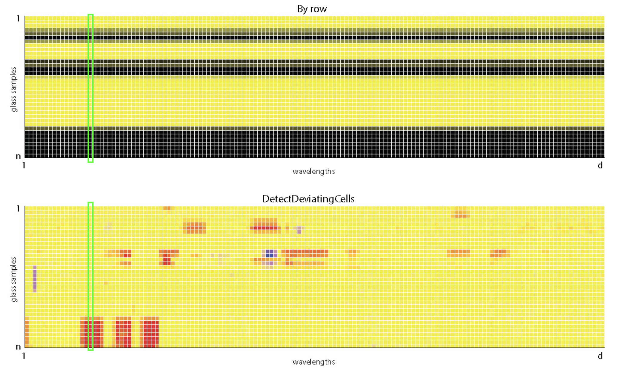
Data: n = 180 archeological glass spectra with d = 750 wavelengths (Detecting Deviating Data Cells, Rousseeuw & Van Den Bossche, Technometrics 2018)

Looking at the values of the wavelength V169:

Robustness vs Efficiency

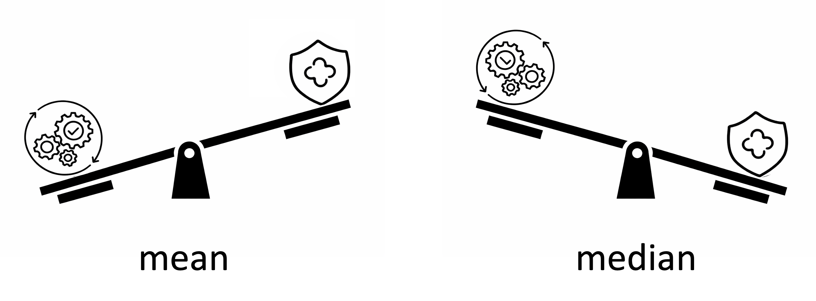
Can we achieve robustness without loss of efficiency?

Which distribution generated the data?

Suppose that we know which distribution generated the data but we don’t know it’s center, how can we estimated?

Maximum Likelihood Estimator (MLE)

MLE chooses the center \(\mu\) that makes the observed data most probable under the assumed distribution
The Normal distribution is given by:

\[ f(x;\mu,\sigma) = \frac{1}{\sqrt{2\pi}\,\sigma} \exp\!\left( -\frac{(x-\mu)^2}{2\sigma^2} \right) \]

If we assume that the data is Normally distributed, with \(\sigma = 1\) but \(\mu\) unknown, and with some math, we can show that

\[ \hat{\mu}_{\text{MLE}} = \arg\min_{\mu} \sum_{i=1}^n \!(x_i-\mu)^2 \]

The MLE

\[ \hat{\mu}_{\text{MLE}} = \arg\min_{\mu} \sum_{i=1}^n \!(x_i-\mu)^2 \]

Definition

\(\arg\min_{\mu}\) denotes the value of \(\mu\) that minimizes the sum of squared deviations.

Using Calculus, it is easy to show that

\[\hat{\mu}_{\text{MLE}} = \bar{x}\]

when the data is Normal, the MLE is the sample mean

Similarly, we can show that

when the data is double exponential, the MLE is the sample median

But in general, we don’t know the distribution. It may even be a mixture of distributions that generated contaminated data!

The M-estimators

\[ \hat{\mu}_{\text{MLE}} = \arg\min_{\mu} \sum_{i=1}^n \!(x_i-\mu)^2 \] From the MLE to the M-estimator:

\[ \hat{\mu}_M = \arg\min_{\mu} \sum_{i=1}^n \rho(x_i-\mu) \]

Instead of of squaring deviations, we measure them with a differentiable function \(\rho\)

The \(\rho\) function

Robustness vs Efficiency		\(\rho(r)\)		Estimator
		square		Mean
		absolute		Median
		differenciable?		M-estimator

Different \(M\)-estimators of location have been proposed:

# grid
x <- seq(-6, 6, length.out = 400)

df <- tibble(
  x = x,
  Mean     = 0.5 * x^2,
  Median   = abs(x),
  Huber    = Mpsi(x, psi = "huber",    cc = 1.5,   deriv = -1),
  Bisquare = Mpsi(x, psi = "bisquare", cc = 4.685, deriv = -1)) |>
  pivot_longer(-x, names_to = "type", values_to = "rho") |>
  mutate(type = factor(type, levels = c("Mean", "Huber", "Median", "Bisquare"))
  )

cc_lines <- tibble(
  type = c("Huber", "Huber", "Bisquare", "Bisquare"),
  xint = c(-1.5, 1.5, -4.685, 4.685)) |>
  mutate(type = factor(type, levels = levels(df$type)))

rho_plot <- ggplot(df, aes(x, rho)) +
  geom_line(linewidth = 1) +
  geom_vline(
    data = cc_lines,
    aes(xintercept = xint),
    linetype = "dashed",
    linewidth = 0.6) +
  facet_wrap(~ type, ncol = 2, scales = "free_y") +
  labs(x = "x", y = expression(rho(x))) +
  theme_minimal(base_size = 14)

Tuning constants

The Huber M-estimator: quadratic near 0 and linear in the tails
The tuning constant (c) marks the change and controls the robustness–efficiency trade-off.

Table shows values V, such that `Var(est) = V / n`

c	Estimator	Efficiency	\(\varepsilon=0\)	\(\varepsilon=0.1\)
0	Median	0.64	1.571	1.897
1.0	Huber M	0.90	1.107	1.443
1.345	Huber M	0.95	1.047	1.439
2.0	Huber M	0.99	1.010	1.549
\(\infty\)	Mean	1	1.000	10.900

For \(\sigma\) unknown

In practice, \(\sigma\) (SD of data, aka scale) is usually unknown and must be estimated from the data.

The SD is efficient but not robust to outliers
The MAD (median absolute deviation) is highly robust:

\[1.4826 \, \text{median}(|x_i - \text{median}|)\]

We can define an M-estimator for the scale (M-scale)
We can also estimate location and scale jointly via M-estimation

In R

mad(x) computes the MAD
locScaleM(x) in RobStatTM computes Huber and bisquare M-estimators (jointly for location and scale) at various asymptiotic efficiency values

Simulation design

Clean data: Generate a sample of size 100 from a Normal distribution with mean 0 and standard deviation 1
Contaminated data: Generate a sample of size 100, with 90% from \(\mathcal{N}(0,1)\) and 10% from \(\mathcal{N}(0,10)\)
Compute the mean and the median
Repeat 10000 times
Approximate the variance of the estimators

set.seed(200)

rcont_norm <- function(n, eps = 0.10, mu0 = 0, sigma0 = 1, sigma1 = 10) {
  x <- rnorm(n, mean = mu0, sd = sigma0)
  
  k <- ceiling(eps * n)              
  if (k > 0) {
    idx <- sample(1:n, k)
    x[idx] <- rnorm(k, mean = mu0, sd = sigma1)
  }
  x
}

#no contamination

eps = 0
sim <- replicate(1000, {
    x <- rcont_norm(100, eps = eps)
    c(
      Mean     = mean(x),
      Median   = median(x),
      Bisquare_3.44 = locScaleM(x, psi="bisquare", eff=0.85)$mu,
      Bisquare_4.68 = locScaleM(x, psi="bisquare", eff=0.95)$mu
    )
  })

  
var0  <- apply(t(sim), 2, var)

#with contamination
eps = 0.20
sim <- replicate(1000, {
    x <- rcont_norm(100, eps = eps)
    c(
      Mean     = mean(x),
      Median   = median(x),
      Bisquare_3.44 = locScaleM(x, psi="bisquare", eff=0.85)$mu,
      Bisquare_4.68 = locScaleM(x, psi="bisquare", eff=0.95)$mu
    )
  })
  
var20 <- apply(t(sim), 2, var)

Approximated Variance of the Bisquare M-estimator

Estimator	Eff	ε = 0	ε = 0.20
Mean	1.00	0.010	0.208
Median	0.64	0.016	0.023
Bisquare_3.44	0.85	0.012	0.015
Bisquare_4.68	0.95	0.011	0.016

Detecting Outliers

How do we know if the data contains outliers?

The 3-\(\sigma\) rule

Classical rule: observations far from the mean are considered outliers
What is “far”? We can measure

\[z_i = \frac{x_i-\bar x}{s}\]

Flag as outlier if: \(|z_i| > 3\)

iClicker 1: interpretation of the rule

With the 3-\(\sigma\) rule:

\[|z_i| = \left|\frac{x_i-\bar x}{s}\right| > 3 \]

an observation is flagged as an outlier if

A. The observation is more than 3 standard deviations from the mean
B. The observation is in the largest 3% of the data
C. The observation is larger than 3 times the mean
D. The observation is more than 3 units from the median

iClicker 2: use the rule

Which points are flagged as outliers using the 3-\(\sigma\) rule?

x <- c(-2,-1,0,1,2,13,20)

mean(x); sd(x)

[1] 4.714286

[1] 8.40068

z  <- (x-mean(x))/sd(x)
z

[1] -0.7992550 -0.6802170 -0.5611790 -0.4421411 -0.3231031  0.9863147  1.8195805

A. Both \(x=13\) and \(x=20\) are flagged
B. Only \(x=20\) is flagged
C. All points are flagged
D. None of points are flagged

Masking

The mean and SD are sensitive to outliers
Extreme observations pull the mean toward them and inflate the standard deviation, reducing their standardized distance
Robust alternative: use median and MAD (or other robust loc-scale estimators)

Robust z-score:

\[z_i^{rob} = \frac{x_i-\text{median}}{\text{MAD}}\]

Rule: \(|z_i^{rob}| > 3\)

iClicker 3: use the robust rule

Which points are flagged as outliers using the 3-\(\sigma\) rule?

x <- c(-2,-1,0,1,2,13,20)

median(x); mad(x)

[1] 1

[1] 2.9652

z  <- (x-median(x))/mad(x)
z

[1] -1.0117361 -0.6744908 -0.3372454  0.0000000  0.3372454  4.0469446  6.4076622

A. Both \(x=13\) and \(x=20\) are flagged
B. Only \(x=20\) is flagged
C. All points are flagged
D. None of points are flagged

Key Takeaways

Classical estimators (mean, SD) are highly sensitive to outliers
Robust estimators reduce the influence of extreme observations
M-estimators provide a flexible compromise between efficiency and robustness
The tuning constant controls this trade-off
Robust methods improve both estimation and outlier detection

Outliers II

Attribution

Review

Univariate estimators

Robustness vs Efficiency

Can we achieve robustness without loss of efficiency?

Which distribution generated the data?

Maximum Likelihood Estimator (MLE)

The MLE

when the data is Normal, the MLE is the sample mean

when the data is double exponential, the MLE is the sample median

The M-estimators

Instead of of squaring deviations, we measure them with a differentiable function \(\rho\)

The \(\rho\) function

Tuning constants

Table shows values V, such that Var(est) = V / n

For \(\sigma\) unknown

In R

Simulation design

Approximated Variance of the Bisquare M-estimator

Detecting Outliers

The 3-\(\sigma\) rule

iClicker 1: interpretation of the rule

iClicker 2: use the rule

Masking

Robust z-score:

iClicker 3: use the robust rule

Key Takeaways

Table shows values V, such that `Var(est) = V / n`