 Data Science
Chapter 6 Classification II: evaluation & tuning
6.1 Overview
This chapter continues the introduction to predictive modeling through classification. While the previous chapter covered training and data preprocessing, this chapter focuses on how to evaluate the performance of a classifier, as well as how to improve the classifier (where possible) to maximize its accuracy.
6.2 Chapter learning objectives
By the end of the chapter, readers will be able to do the following:
- Describe what training, validation, and test data sets are and how they are used in classification.
- Split data into training, validation, and test data sets.
- Describe what a random seed is and its importance in reproducible data analysis.
- Set the random seed in R using the
set.seedfunction. - Describe and interpret accuracy, precision, recall, and confusion matrices.
- Evaluate classification accuracy, precision, and recall in R using a test set, a single validation set, and cross-validation.
- Produce a confusion matrix in R.
- Choose the number of neighbors in a K-nearest neighbors classifier by maximizing estimated cross-validation accuracy.
- Describe underfitting and overfitting, and relate it to the number of neighbors in K-nearest neighbors classification.
- Describe the advantages and disadvantages of the K-nearest neighbors classification algorithm.
6.3 Evaluating performance
Sometimes our classifier might make the wrong prediction. A classifier does not need to be right 100% of the time to be useful, though we don’t want the classifier to make too many wrong predictions. How do we measure how “good” our classifier is? Let’s revisit the breast cancer images data (Street, Wolberg, and Mangasarian 1993) and think about how our classifier will be used in practice. A biopsy will be performed on a new patient’s tumor, the resulting image will be analyzed, and the classifier will be asked to decide whether the tumor is benign or malignant. The key word here is new: our classifier is “good” if it provides accurate predictions on data not seen during training, as this implies that it has actually learned about the relationship between the predictor variables and response variable, as opposed to simply memorizing the labels of individual training data examples. But then, how can we evaluate our classifier without visiting the hospital to collect more tumor images?
The trick is to split the data into a training set and test set (Figure 6.1) and use only the training set when building the classifier. Then, to evaluate the performance of the classifier, we first set aside the labels from the test set, and then use the classifier to predict the labels in the test set. If our predictions match the actual labels for the observations in the test set, then we have some confidence that our classifier might also accurately predict the class labels for new observations without known class labels.
Note: If there were a golden rule of machine learning, it might be this: you cannot use the test data to build the model! If you do, the model gets to “see” the test data in advance, making it look more accurate than it really is. Imagine how bad it would be to overestimate your classifier’s accuracy when predicting whether a patient’s tumor is malignant or benign!
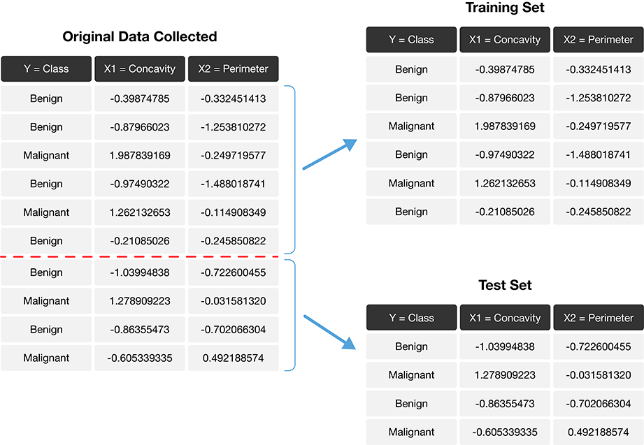
Figure 6.1: Splitting the data into training and testing sets.
How exactly can we assess how well our predictions match the actual labels for the observations in the test set? One way we can do this is to calculate the prediction accuracy. This is the fraction of examples for which the classifier made the correct prediction. To calculate this, we divide the number of correct predictions by the number of predictions made. The process for assessing if our predictions match the actual labels in the test set is illustrated in Figure 6.2.
\[\mathrm{accuracy} = \frac{\mathrm{number \; of \; correct \; predictions}}{\mathrm{total \; number \; of \; predictions}}\]
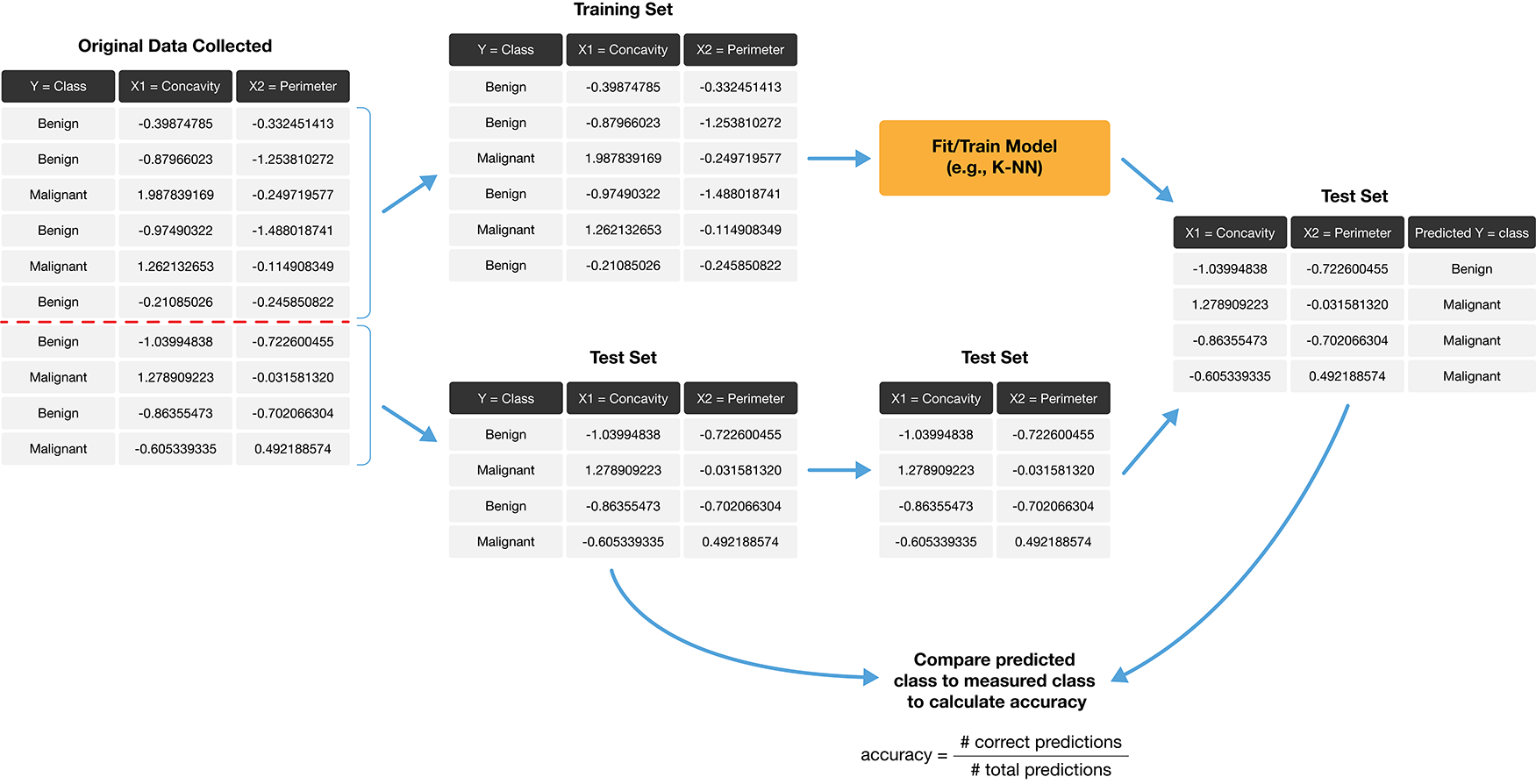
Figure 6.2: Process for splitting the data and finding the prediction accuracy.
Accuracy is a convenient, general-purpose way to summarize the performance of a classifier with a single number. But prediction accuracy by itself does not tell the whole story. In particular, accuracy alone only tells us how often the classifier makes mistakes in general, but does not tell us anything about the kinds of mistakes the classifier makes. A more comprehensive view of performance can be obtained by additionally examining the confusion matrix. The confusion matrix shows how many test set labels of each type are predicted correctly and incorrectly, which gives us more detail about the kinds of mistakes the classifier tends to make. Table 6.1 shows an example of what a confusion matrix might look like for the tumor image data with a test set of 65 observations.
| Actually Malignant | Actually Benign | |
|---|---|---|
| Predicted Malignant | 1 | 4 |
| Predicted Benign | 3 | 57 |
In the example in Table 6.1, we see that there was 1 malignant observation that was correctly classified as malignant (top left corner), and 57 benign observations that were correctly classified as benign (bottom right corner). However, we can also see that the classifier made some mistakes: it classified 3 malignant observations as benign, and 4 benign observations as malignant. The accuracy of this classifier is roughly 89%, given by the formula
\[\mathrm{accuracy} = \frac{\mathrm{number \; of \; correct \; predictions}}{\mathrm{total \; number \; of \; predictions}} = \frac{1+57}{1+57+4+3} = 0.892.\]
But we can also see that the classifier only identified 1 out of 4 total malignant tumors; in other words, it misclassified 75% of the malignant cases present in the data set! In this example, misclassifying a malignant tumor is a potentially disastrous error, since it may lead to a patient who requires treatment not receiving it. Since we are particularly interested in identifying malignant cases, this classifier would likely be unacceptable even with an accuracy of 89%.
Focusing more on one label than the other is common in classification problems. In such cases, we typically refer to the label we are more interested in identifying as the positive label, and the other as the negative label. In the tumor example, we would refer to malignant observations as positive, and benign observations as negative. We can then use the following terms to talk about the four kinds of prediction that the classifier can make, corresponding to the four entries in the confusion matrix:
- True Positive: A malignant observation that was classified as malignant (top left in Table 6.1).
- False Positive: A benign observation that was classified as malignant (top right in Table 6.1).
- True Negative: A benign observation that was classified as benign (bottom right in Table 6.1).
- False Negative: A malignant observation that was classified as benign (bottom left in Table 6.1).
A perfect classifier would have zero false negatives and false positives (and therefore, 100% accuracy). However, classifiers in practice will almost always make some errors. So you should think about which kinds of error are most important in your application, and use the confusion matrix to quantify and report them. Two commonly used metrics that we can compute using the confusion matrix are the precision and recall of the classifier. These are often reported together with accuracy. Precision quantifies how many of the positive predictions the classifier made were actually positive. Intuitively, we would like a classifier to have a high precision: for a classifier with high precision, if the classifier reports that a new observation is positive, we can trust that the new observation is indeed positive. We can compute the precision of a classifier using the entries in the confusion matrix, with the formula
\[\mathrm{precision} = \frac{\mathrm{number \; of \; correct \; positive \; predictions}}{\mathrm{total \; number \; of \; positive \; predictions}}.\]
Recall quantifies how many of the positive observations in the test set were identified as positive. Intuitively, we would like a classifier to have a high recall: for a classifier with high recall, if there is a positive observation in the test data, we can trust that the classifier will find it. We can also compute the recall of the classifier using the entries in the confusion matrix, with the formula
\[\mathrm{recall} = \frac{\mathrm{number \; of \; correct \; positive \; predictions}}{\mathrm{total \; number \; of \; positive \; test \; set \; observations}}.\]
In the example presented in Table 6.1, we have that the precision and recall are
\[\mathrm{precision} = \frac{1}{1+4} = 0.20, \quad \mathrm{recall} = \frac{1}{1+3} = 0.25.\]
So even with an accuracy of 89%, the precision and recall of the classifier were both relatively low. For this data analysis context, recall is particularly important: if someone has a malignant tumor, we certainly want to identify it. A recall of just 25% would likely be unacceptable!
Note: It is difficult to achieve both high precision and high recall at the same time; models with high precision tend to have low recall and vice versa. As an example, we can easily make a classifier that has perfect recall: just always guess positive! This classifier will of course find every positive observation in the test set, but it will make lots of false positive predictions along the way and have low precision. Similarly, we can easily make a classifier that has perfect precision: never guess positive! This classifier will never incorrectly identify an obsevation as positive, but it will make a lot of false negative predictions along the way. In fact, this classifier will have 0% recall! Of course, most real classifiers fall somewhere in between these two extremes. But these examples serve to show that in settings where one of the classes is of interest (i.e., there is a positive label), there is a trade-off between precision and recall that one has to make when designing a classifier.
6.4 Randomness and seeds
Beginning in this chapter, our data analyses will often involve the use of randomness. We use randomness any time we need to make a decision in our analysis that needs to be fair, unbiased, and not influenced by human input. For example, in this chapter, we need to split a data set into a training set and test set to evaluate our classifier. We certainly do not want to choose how to split the data ourselves by hand, as we want to avoid accidentally influencing the result of the evaluation. So instead, we let R randomly split the data. In future chapters we will use randomness in many other ways, e.g., to help us select a small subset of data from a larger data set, to pick groupings of data, and more.
However, the use of randomness runs counter to one of the main
tenets of good data analysis practice: reproducibility. Recall that a reproducible
analysis produces the same result each time it is run; if we include randomness
in the analysis, would we not get a different result each time?
The trick is that in R—and other programming languages—randomness
is not actually random! Instead, R uses a random number generator that
produces a sequence of numbers that
are completely determined by a
seed value. Once you set the seed value
using the set.seed function, everything after that point may look random,
but is actually totally reproducible. As long as you pick the same seed
value, you get the same result!
Let’s use an example to investigate how seeds work in R. Say we want
to randomly pick 10 numbers from 0 to 9 in R using the sample function,
but we want it to be reproducible. Before using the sample function,
we call set.seed, and pass it any integer as an argument.
Here, we pass in the number 1.
## [1] 8 3 6 0 1 6 1 2 0 4You can see that random_numbers1 is a list of 10 numbers
from 0 to 9 that, from all appearances, looks random. If
we run the sample function again, we will
get a fresh batch of 10 numbers that also look random.
## [1] 4 9 5 9 6 8 4 4 8 8If we want to force R to produce the same sequences of random numbers,
we can simply call the set.seed function again with the same argument
value.
## [1] 8 3 6 0 1 6 1 2 0 4## [1] 4 9 5 9 6 8 4 4 8 8Notice that after setting the seed, we get the same two sequences of numbers in the same order. random_numbers1 and random_numbers1_again produce the same sequence of numbers, and the same can be said about random_numbers2 and random_numbers2_again. And if we choose
a different value for the seed—say, 4235—we
obtain a different sequence of random numbers.
set.seed(4235)
random_numbers1_different <- sample(0:9, 10, replace = TRUE)
random_numbers1_different
## [1] 8 3 1 4 6 8 8 4 1 7## [1] 3 7 8 2 8 8 6 3 3 8In other words, even though the sequences of numbers that R is generating look random, they are totally determined when we set a seed value!
So what does this mean for data analysis? Well, sample is certainly
not the only function that uses randomness in R. Many of the functions
that we use in tidymodels, tidyverse, and beyond use randomness—some of them
without even telling you about it. So at the beginning of every data analysis you
do, right after loading packages, you should call the set.seed function and
pass it an integer that you pick.
Also note that when R starts up, it creates its own seed to use. So if you do not
explicitly call the set.seed function in your code, your results will
likely not be reproducible.
And finally, be careful to set the seed only once at the beginning of a data
analysis. Each time you set the seed, you are inserting your own human input,
thereby influencing the analysis. If you use set.seed many times
throughout your analysis, the randomness that R uses will not look
as random as it should.
In summary: if you want your analysis to be reproducible, i.e., produce the same result each time you
run it, make sure to use set.seed exactly once at the beginning of the analysis.
Different argument values in set.seed lead to different patterns of randomness, but as long as
you pick the same argument value your result will be the same.
In the remainder of the textbook, we will set the seed once at the beginning of each chapter.
6.5 Evaluating performance with tidymodels
Back to evaluating classifiers now!
In R, we can use the tidymodels package not only to perform K-nearest neighbors
classification, but also to assess how well our classification worked.
Let’s work through an example of how to use tools from tidymodels to evaluate a classifier
using the breast cancer data set from the previous chapter.
We begin the analysis by loading the packages we require,
reading in the breast cancer data,
and then making a quick scatter plot visualization of
tumor cell concavity versus smoothness colored by diagnosis in Figure 6.3.
You will also notice that we set the random seed here at the beginning of the analysis
using the set.seed function, as described in Section 6.4.
# load packages
library(tidyverse)
library(tidymodels)

# set the seed
set.seed(1)

# load data
cancer <- read_csv("data/wdbc_unscaled.csv") |>
  # convert the character Class variable to the factor datatype
  mutate(Class = as_factor(Class))  |>
  # rename the factor values to be more readable
  mutate(Class = fct_recode(Class, "Malignant" = "M", "Benign" = "B"))

# create scatter plot of tumor cell concavity versus smoothness,
# labeling the points be diagnosis class
perim_concav <- cancer |>
  ggplot(aes(x = Smoothness, y = Concavity, color = Class)) +
  geom_point(alpha = 0.5) +
  labs(color = "Diagnosis") +
  scale_color_manual(values = c("darkorange", "steelblue")) +
  theme(text = element_text(size = 12))

perim_concav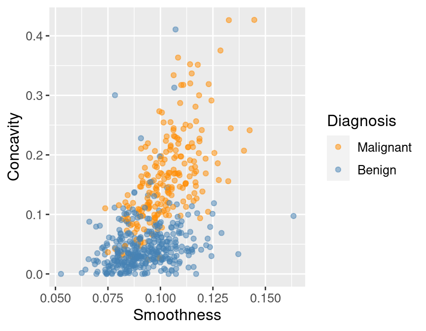
Figure 6.3: Scatter plot of tumor cell concavity versus smoothness colored by diagnosis label.
6.5.1 Create the train / test split
Once we have decided on a predictive question to answer and done some preliminary exploration, the very next thing to do is to split the data into the training and test sets. Typically, the training set is between 50% and 95% of the data, while the test set is the remaining 5% to 50%; the intuition is that you want to trade off between training an accurate model (by using a larger training data set) and getting an accurate evaluation of its performance (by using a larger test data set). Here, we will use 75% of the data for training, and 25% for testing.
The initial_split function from tidymodels handles the procedure of splitting
the data for us. It also applies two very important steps when splitting to ensure
that the accuracy estimates from the test data are reasonable. First, it
shuffles the data before splitting, which ensures that any ordering present
in the data does not influence the data that ends up in the training and testing sets.
Second, it stratifies the data by the class label, to ensure that roughly
the same proportion of each class ends up in both the training and testing sets. For example,
in our data set, roughly 63% of the
observations are from the benign class, and 37% are from the malignant class,
so initial_split ensures that roughly 63% of the training data are benign,
37% of the training data are malignant,
and the same proportions exist in the testing data.
Let’s use the initial_split function to create the training and testing sets.
We will specify that prop = 0.75 so that 75% of our original data set ends up
in the training set. We will also set the strata argument to the categorical label variable
(here, Class) to ensure that the training and testing subsets contain the
right proportions of each category of observation.
The training and testing functions then extract the training and testing
data sets into two separate data frames.
Note that the initial_split function uses randomness, but since we set the
seed earlier in the chapter, the split will be reproducible.
cancer_split <- initial_split(cancer, prop = 0.75, strata = Class)
cancer_train <- training(cancer_split)
cancer_test <- testing(cancer_split)## Rows: 426
## Columns: 12
## $ ID <dbl> 8510426, 8510653, 8510824, 854941, 85713702, 857155,…
## $ Class <fct> Benign, Benign, Benign, Benign, Benign, Benign, Beni…
## $ Radius <dbl> 13.540, 13.080, 9.504, 13.030, 8.196, 12.050, 13.490…
## $ Texture <dbl> 14.36, 15.71, 12.44, 18.42, 16.84, 14.63, 22.30, 21.…
## $ Perimeter <dbl> 87.46, 85.63, 60.34, 82.61, 51.71, 78.04, 86.91, 74.…
## $ Area <dbl> 566.3, 520.0, 273.9, 523.8, 201.9, 449.3, 561.0, 427…
## $ Smoothness <dbl> 0.09779, 0.10750, 0.10240, 0.08983, 0.08600, 0.10310…
## $ Compactness <dbl> 0.08129, 0.12700, 0.06492, 0.03766, 0.05943, 0.09092…
## $ Concavity <dbl> 0.066640, 0.045680, 0.029560, 0.025620, 0.015880, 0.…
## $ Concave_Points <dbl> 0.047810, 0.031100, 0.020760, 0.029230, 0.005917, 0.…
## $ Symmetry <dbl> 0.1885, 0.1967, 0.1815, 0.1467, 0.1769, 0.1675, 0.18…
## $ Fractal_Dimension <dbl> 0.05766, 0.06811, 0.06905, 0.05863, 0.06503, 0.06043…## Rows: 143
## Columns: 12
## $ ID <dbl> 842517, 84300903, 84501001, 84610002, 848406, 848620…
## $ Class <fct> Malignant, Malignant, Malignant, Malignant, Malignan…
## $ Radius <dbl> 20.570, 19.690, 12.460, 15.780, 14.680, 16.130, 19.8…
## $ Texture <dbl> 17.77, 21.25, 24.04, 17.89, 20.13, 20.68, 22.15, 14.…
## $ Perimeter <dbl> 132.90, 130.00, 83.97, 103.60, 94.74, 108.10, 130.00…
## $ Area <dbl> 1326.0, 1203.0, 475.9, 781.0, 684.5, 798.8, 1260.0, …
## $ Smoothness <dbl> 0.08474, 0.10960, 0.11860, 0.09710, 0.09867, 0.11700…
## $ Compactness <dbl> 0.07864, 0.15990, 0.23960, 0.12920, 0.07200, 0.20220…
## $ Concavity <dbl> 0.08690, 0.19740, 0.22730, 0.09954, 0.07395, 0.17220…
## $ Concave_Points <dbl> 0.070170, 0.127900, 0.085430, 0.066060, 0.052590, 0.…
## $ Symmetry <dbl> 0.1812, 0.2069, 0.2030, 0.1842, 0.1586, 0.2164, 0.15…
## $ Fractal_Dimension <dbl> 0.05667, 0.05999, 0.08243, 0.06082, 0.05922, 0.07356…We can see from glimpse in the code above that the training set contains 426
observations, while the test set contains 143 observations. This corresponds to
a train / test split of 75% / 25%, as desired. Recall from Chapter 5
that we use the glimpse function to view data with a large number of columns,
as it prints the data such that the columns go down the page (instead of across).
We can use group_by and summarize to find the percentage of malignant and benign classes
in cancer_train and we see about 63% of the training
data are benign and 37%
are malignant, indicating that our class proportions were roughly preserved when we split the data.
cancer_proportions <- cancer_train |>
                      group_by(Class) |>
                      summarize(n = n()) |>
                      mutate(percent = 100*n/nrow(cancer_train))

cancer_proportions
## # A tibble: 2 × 3
## Class n percent
## <fct> <int> <dbl>
## 1 Malignant 159 37.3
## 2 Benign 267 62.76.5.2 Preprocess the data
As we mentioned in the last chapter, K-nearest neighbors is sensitive to the scale of the predictors, so we should perform some preprocessing to standardize them. An additional consideration we need to take when doing this is that we should create the standardization preprocessor using only the training data. This ensures that our test data does not influence any aspect of our model training. Once we have created the standardization preprocessor, we can then apply it separately to both the training and test data sets.
Fortunately, the recipe framework from tidymodels helps us handle
this properly. Below we construct and prepare the recipe using only the training
data (due to data = cancer_train in the first line).
6.5.3 Train the classifier
Now that we have split our original data set into training and test sets, we
can create our K-nearest neighbors classifier with only the training set using
the technique we learned in the previous chapter. For now, we will just choose
the number \(K\) of neighbors to be 3, and use concavity and smoothness as the
predictors. As before we need to create a model specification, combine
the model specification and recipe into a workflow, and then finally
use fit with the training data cancer_train to build the classifier.
knn_spec <- nearest_neighbor(weight_func = "rectangular", neighbors = 3) |>
set_engine("kknn") |>
set_mode("classification")
knn_fit <- workflow() |>
add_recipe(cancer_recipe) |>
add_model(knn_spec) |>
fit(data = cancer_train)
knn_fit## ══ Workflow [trained] ══════════
## Preprocessor: Recipe
## Model: nearest_neighbor()
##
## ── Preprocessor ──────────
## 2 Recipe Steps
##
## • step_scale()
## • step_center()
##
## ── Model ──────────
##
## Call:
## kknn::train.kknn(formula = ..y ~ ., data = data, ks = min_rows(3, data, 5),
## kernel = ~"rectangular")
##
## Type of response variable: nominal
## Minimal misclassification: 0.1126761
## Best kernel: rectangular
## Best k: 36.5.4 Predict the labels in the test set
Now that we have a K-nearest neighbors classifier object, we can use it to
predict the class labels for our test set. We use the bind_cols to add the
column of predictions to the original test data, creating the
cancer_test_predictions data frame. The Class variable contains the actual
diagnoses, while the .pred_class contains the predicted diagnoses from the
classifier.
cancer_test_predictions <- predict(knn_fit, cancer_test) |>
bind_cols(cancer_test)
cancer_test_predictions## # A tibble: 143 × 13
## .pred_class ID Class Radius Texture Perimeter Area Smoothness
## <fct> <dbl> <fct> <dbl> <dbl> <dbl> <dbl> <dbl>
## 1 Benign 842517 Malignant 20.6 17.8 133. 1326 0.0847
## 2 Malignant 84300903 Malignant 19.7 21.2 130 1203 0.110
## 3 Malignant 84501001 Malignant 12.5 24.0 84.0 476. 0.119
## 4 Malignant 84610002 Malignant 15.8 17.9 104. 781 0.0971
## 5 Benign 848406 Malignant 14.7 20.1 94.7 684. 0.0987
## 6 Malignant 84862001 Malignant 16.1 20.7 108. 799. 0.117
## 7 Malignant 849014 Malignant 19.8 22.2 130 1260 0.0983
## 8 Malignant 8511133 Malignant 15.3 14.3 102. 704. 0.107
## 9 Malignant 852552 Malignant 16.6 21.4 110 905. 0.112
## 10 Malignant 853612 Malignant 11.8 18.7 77.9 441. 0.111
## # ℹ 133 more rows
## # ℹ 5 more variables: Compactness <dbl>, Concavity <dbl>, Concave_Points <dbl>,
## # Symmetry <dbl>, Fractal_Dimension <dbl>6.5.5 Evaluate performance
Finally, we can assess our classifier’s performance. First, we will examine
accuracy. To do this we use the
metrics function from tidymodels,
specifying the truth and estimate arguments:
cancer_test_predictions |>
metrics(truth = Class, estimate = .pred_class) |>
filter(.metric == "accuracy")## # A tibble: 1 × 3
## .metric .estimator .estimate
## <chr> <chr> <dbl>
## 1 accuracy binary 0.853In the metrics data frame, we filtered the .metric column since we are
interested in the accuracy row. Other entries involve other metrics that
are beyond the scope of this book. Looking at the value of the .estimate variable
shows that the estimated accuracy of the classifier on the test data
was 85%.
To compute the precision and recall, we can use the precision and recall functions
from tidymodels. We first check the order of the
labels in the Class variable using the levels function:
## [1] "Malignant" "Benign"This shows that "Malignant" is the first level. Therefore we will set
the truth and estimate arguments to Class and .pred_class as before,
but also specify that the “positive” class corresponds to the first factor level via event_level="first".
If the labels were in the other order, we would instead use event_level="second".
## # A tibble: 1 × 3
## .metric .estimator .estimate
## <chr> <chr> <dbl>
## 1 precision binary 0.767## # A tibble: 1 × 3
## .metric .estimator .estimate
## <chr> <chr> <dbl>
## 1 recall binary 0.868The output shows that the estimated precision and recall of the classifier on the test data was
77% and 87%, respectively.
Finally, we can look at the confusion matrix for the classifier using the conf_mat function.
## Truth
## Prediction Malignant Benign
## Malignant 46 14
## Benign 7 76The confusion matrix shows 46 observations were correctly predicted as malignant, and 76 were correctly predicted as benign. It also shows that the classifier made some mistakes; in particular, it classified 7 observations as benign when they were actually malignant, and 14 observations as malignant when they were actually benign. Using our formulas from earlier, we see that the accuracy, precision, and recall agree with what R reported.
\[\mathrm{accuracy} = \frac{\mathrm{number \; of \; correct \; predictions}}{\mathrm{total \; number \; of \; predictions}} = \frac{46+76}{46+76+14+7} = 0.853\]
\[\mathrm{precision} = \frac{\mathrm{number \; of \; correct \; positive \; predictions}}{\mathrm{total \; number \; of \; positive \; predictions}} = \frac{46}{46 + 14} = 0.767\]
\[\mathrm{recall} = \frac{\mathrm{number \; of \; correct \; positive \; predictions}}{\mathrm{total \; number \; of \; positive \; test \; set \; observations}} = \frac{46}{46+7} = 0.868\]
6.5.6 Critically analyze performance
We now know that the classifier was 85% accurate on the test data set, and had a precision of 77% and a recall of 87%. That sounds pretty good! Wait, is it good? Or do we need something higher?
In general, a good value for accuracy (as well as precision and recall, if applicable) depends on the application; you must critically analyze your accuracy in the context of the problem you are solving. For example, if we were building a classifier for a kind of tumor that is benign 99% of the time, a classifier with 99% accuracy is not terribly impressive (just always guess benign!). And beyond just accuracy, we need to consider the precision and recall: as mentioned earlier, the kind of mistake the classifier makes is important in many applications as well. In the previous example with 99% benign observations, it might be very bad for the classifier to predict “benign” when the actual class is “malignant” (a false negative), as this might result in a patient not receiving appropriate medical attention. In other words, in this context, we need the classifier to have a high recall. On the other hand, it might be less bad for the classifier to guess “malignant” when the actual class is “benign” (a false positive), as the patient will then likely see a doctor who can provide an expert diagnosis. In other words, we are fine with sacrificing some precision in the interest of achieving high recall. This is why it is important not only to look at accuracy, but also the confusion matrix.
However, there is always an easy baseline that you can compare to for any classification problem: the majority classifier. The majority classifier always guesses the majority class label from the training data, regardless of the predictor variables’ values. It helps to give you a sense of scale when considering accuracies. If the majority classifier obtains a 90% accuracy on a problem, then you might hope for your K-nearest neighbors classifier to do better than that. If your classifier provides a significant improvement upon the majority classifier, this means that at least your method is extracting some useful information from your predictor variables. Be careful though: improving on the majority classifier does not necessarily mean the classifier is working well enough for your application.
As an example, in the breast cancer data, recall the proportions of benign and malignant observations in the training data are as follows:
## # A tibble: 2 × 3
##   Class         n percent
##   <fct>     <int>   <dbl>
## 1 Malignant   159    37.3
## 2 Benign 267 62.7Since the benign class represents the majority of the training data, the majority classifier would always predict that a new observation is benign. The estimated accuracy of the majority classifier is usually fairly close to the majority class proportion in the training data. In this case, we would suspect that the majority classifier will have an accuracy of around 63%. The K-nearest neighbors classifier we built does quite a bit better than this, with an accuracy of 85%. This means that from the perspective of accuracy, the K-nearest neighbors classifier improved quite a bit on the basic majority classifier. Hooray! But we still need to be cautious; in this application, it is likely very important not to misdiagnose any malignant tumors to avoid missing patients who actually need medical care. The confusion matrix above shows that the classifier does, indeed, misdiagnose a significant number of malignant tumors as benign (7 out of 53 malignant tumors, or 13%!). Therefore, even though the accuracy improved upon the majority classifier, our critical analysis suggests that this classifier may not have appropriate performance for the application.
6.6 Tuning the classifier
The vast majority of predictive models in statistics and machine learning have parameters. A parameter is a number you have to pick in advance that determines some aspect of how the model behaves. For example, in the K-nearest neighbors classification algorithm, \(K\) is a parameter that we have to pick that determines how many neighbors participate in the class vote. By picking different values of \(K\), we create different classifiers that make different predictions.
So then, how do we pick the best value of \(K\), i.e., tune the model? And is it possible to make this selection in a principled way? In this book, we will focus on maximizing the accuracy of the classifier. Ideally, we want somehow to maximize the accuracy of our classifier on data it hasn’t seen yet. But we cannot use our test data set in the process of building our model. So we will play the same trick we did before when evaluating our classifier: we’ll split our training data itself into two subsets, use one to train the model, and then use the other to evaluate it. In this section, we will cover the details of this procedure, as well as how to use it to help you pick a good parameter value for your classifier.
And remember: don’t touch the test set during the tuning process. Tuning is a part of model training!
6.6.1 Cross-validation
The first step in choosing the parameter \(K\) is to be able to evaluate the classifier using only the training data. If this is possible, then we can compare the classifier’s performance for different values of \(K\)—and pick the best—using only the training data. As suggested at the beginning of this section, we will accomplish this by splitting the training data, training on one subset, and evaluating on the other. The subset of training data used for evaluation is often called the validation set.
There is, however, one key difference from the train/test split that we performed earlier. In particular, we were forced to make only a single split of the data. This is because at the end of the day, we have to produce a single classifier. If we had multiple different splits of the data into training and testing data, we would produce multiple different classifiers. But while we are tuning the classifier, we are free to create multiple classifiers based on multiple splits of the training data, evaluate them, and then choose a parameter value based on all of the different results. If we just split our overall training data once, our best parameter choice will depend strongly on whatever data was lucky enough to end up in the validation set. Perhaps using multiple different train/validation splits, we’ll get a better estimate of accuracy, which will lead to a better choice of the number of neighbors \(K\) for the overall set of training data.
Let’s investigate this idea in R! In particular, we will generate five different train/validation splits of our overall training data, train five different K-nearest neighbors models, and evaluate their accuracy. We will start with just a single split.
# create the 25/75 split of the training data into training and validation
cancer_split <- initial_split(cancer_train, prop = 0.75, strata = Class)
cancer_subtrain <- training(cancer_split)
cancer_validation <- testing(cancer_split)
# recreate the standardization recipe from before
# (since it must be based on the training data)
cancer_recipe <- recipe(Class ~ Smoothness + Concavity,
data = cancer_subtrain) |>
step_scale(all_predictors()) |>
step_center(all_predictors())
# fit the knn model (we can reuse the old knn_spec model from before)
knn_fit <- workflow() |>
add_recipe(cancer_recipe) |>
add_model(knn_spec) |>
fit(data = cancer_subtrain)
# get predictions on the validation data
validation_predicted <- predict(knn_fit, cancer_validation) |>
bind_cols(cancer_validation)
# compute the accuracy
acc <- validation_predicted |>
metrics(truth = Class, estimate = .pred_class) |>
filter(.metric == "accuracy") |>
select(.estimate) |>
pull()
acc## [1] 0.8598131The accuracy estimate using this split is 86%. Now we repeat the above code 4 more times, which generates 4 more splits. Therefore we get five different shuffles of the data, and therefore five different values for accuracy: 86.0%, 89.7%, 88.8%, 86.0%, 86.9%. None of these values are necessarily “more correct” than any other; they’re just five estimates of the true, underlying accuracy of our classifier built using our overall training data. We can combine the estimates by taking their average (here 87%) to try to get a single assessment of our classifier’s accuracy; this has the effect of reducing the influence of any one (un)lucky validation set on the estimate.
In practice, we don’t use random splits, but rather use a more structured splitting procedure so that each observation in the data set is used in a validation set only a single time. The name for this strategy is cross-validation. In cross-validation, we split our overall training data into \(C\) evenly sized chunks. Then, iteratively use \(1\) chunk as the validation set and combine the remaining \(C-1\) chunks as the training set. This procedure is shown in Figure 6.4. Here, \(C=5\) different chunks of the data set are used, resulting in 5 different choices for the validation set; we call this 5-fold cross-validation.
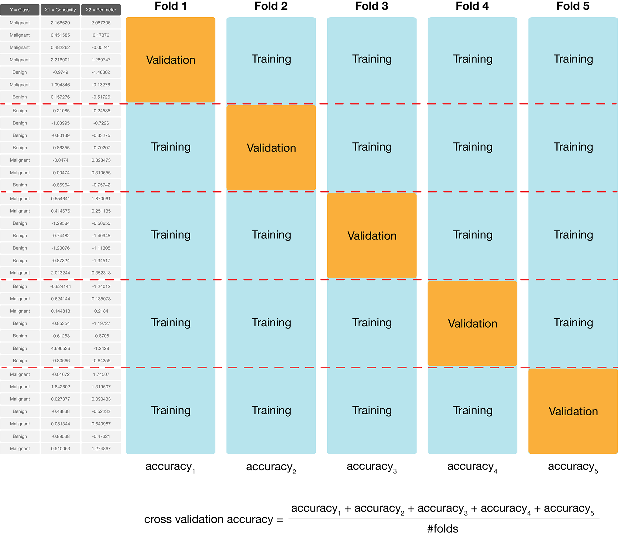
Figure 6.4: 5-fold cross-validation.
To perform 5-fold cross-validation in R with tidymodels, we use another
function: vfold_cv. This function splits our training data into v folds
automatically. We set the strata argument to the categorical label variable
(here, Class) to ensure that the training and validation subsets contain the
right proportions of each category of observation.
## # 5-fold cross-validation using stratification
## # A tibble: 5 × 2
## splits id
## <list> <chr>
## 1 <split [340/86]> Fold1
## 2 <split [340/86]> Fold2
## 3 <split [341/85]> Fold3
## 4 <split [341/85]> Fold4
## 5 <split [342/84]> Fold5Then, when we create our data analysis workflow, we use the fit_resamples function
instead of the fit function for training. This runs cross-validation on each
train/validation split.
# recreate the standardization recipe from before
# (since it must be based on the training data)
cancer_recipe <- recipe(Class ~ Smoothness + Concavity, data = cancer_train) |>
  step_scale(all_predictors()) |>
  step_center(all_predictors())
# fit the knn model (we can reuse the old knn_spec model from before)
knn_fit <- workflow() |>
add_recipe(cancer_recipe) |>
add_model(knn_spec) |>
fit_resamples(resamples = cancer_vfold)
knn_fit## # Resampling results
## # 5-fold cross-validation using stratification
## # A tibble: 5 × 4
## splits id .metrics .notes
## <list> <chr> <list> <list>
## 1 <split [340/86]> Fold1 <tibble [2 × 4]> <tibble [0 × 3]>
## 2 <split [340/86]> Fold2 <tibble [2 × 4]> <tibble [0 × 3]>
## 3 <split [341/85]> Fold3 <tibble [2 × 4]> <tibble [0 × 3]>
## 4 <split [341/85]> Fold4 <tibble [2 × 4]> <tibble [0 × 3]>
## 5 <split [342/84]> Fold5 <tibble [2 × 4]> <tibble [0 × 3]>The collect_metrics function is used to aggregate the mean and standard error
of the classifier’s validation accuracy across the folds. You will find results
related to the accuracy in the row with accuracy listed under the .metric column.
You should consider the mean (mean) to be the estimated accuracy, while the standard
error (std_err) is a measure of how uncertain we are in the mean value. A detailed treatment of this
is beyond the scope of this chapter; but roughly, if your estimated mean is 0.89 and standard
error is 0.02, you can expect the true average accuracy of the
classifier to be somewhere roughly between 87% and 91% (although it may
fall outside this range). You may ignore the other columns in the metrics data frame,
as they do not provide any additional insight.
You can also ignore the entire second row with roc_auc in the .metric column,
as it is beyond the scope of this book.
## # A tibble: 2 × 6
## .metric .estimator mean n std_err .config
## <chr> <chr> <dbl> <int> <dbl> <chr>
## 1 accuracy binary 0.890 5 0.0180 Preprocessor1_Model1
## 2 roc_auc binary 0.925 5 0.0151 Preprocessor1_Model1We can choose any number of folds, and typically the more we use the better our accuracy estimate will be (lower standard error). However, we are limited by computational power: the more folds we choose, the more computation it takes, and hence the more time it takes to run the analysis. So when you do cross-validation, you need to consider the size of the data, the speed of the algorithm (e.g., K-nearest neighbors), and the speed of your computer. In practice, this is a trial-and-error process, but typically \(C\) is chosen to be either 5 or 10. Here we will try 10-fold cross-validation to see if we get a lower standard error:
cancer_vfold <- vfold_cv(cancer_train, v = 10, strata = Class)
vfold_metrics <- workflow() |>
add_recipe(cancer_recipe) |>
add_model(knn_spec) |>
fit_resamples(resamples = cancer_vfold) |>
collect_metrics()
vfold_metrics## # A tibble: 2 × 6
## .metric .estimator mean n std_err .config
## <chr> <chr> <dbl> <int> <dbl> <chr>
## 1 accuracy binary 0.890 10 0.0127 Preprocessor1_Model1
## 2 roc_auc binary 0.913 10 0.0150 Preprocessor1_Model1In this case, using 10-fold instead of 5-fold cross validation did reduce the standard error, although by only an insignificant amount. In fact, due to the randomness in how the data are split, sometimes you might even end up with a higher standard error when increasing the number of folds! We can make the reduction in standard error more dramatic by increasing the number of folds by a large amount. In the following code we show the result when \(C = 50\); picking such a large number of folds often takes a long time to run in practice, so we usually stick to 5 or 10.
cancer_vfold_50 <- vfold_cv(cancer_train, v = 50, strata = Class)
vfold_metrics_50 <- workflow() |>
add_recipe(cancer_recipe) |>
add_model(knn_spec) |>
fit_resamples(resamples = cancer_vfold_50) |>
collect_metrics()
vfold_metrics_50## # A tibble: 2 × 6
## .metric .estimator mean n std_err .config
## <chr> <chr> <dbl> <int> <dbl> <chr>
## 1 accuracy binary 0.884 50 0.00568 Preprocessor1_Model1
## 2 roc_auc binary 0.926 50 0.0148 Preprocessor1_Model16.6.2 Parameter value selection
Using 5- and 10-fold cross-validation, we have estimated that the prediction accuracy of our classifier is somewhere around 89%. Whether that is good or not depends entirely on the downstream application of the data analysis. In the present situation, we are trying to predict a tumor diagnosis, with expensive, damaging chemo/radiation therapy or patient death as potential consequences of misprediction. Hence, we might like to do better than 89% for this application.
In order to improve our classifier, we have one choice of parameter: the number of
neighbors, \(K\). Since cross-validation helps us evaluate the accuracy of our
classifier, we can use cross-validation to calculate an accuracy for each value
of \(K\) in a reasonable range, and then pick the value of \(K\) that gives us the
best accuracy. The tidymodels package collection provides a very simple
syntax for tuning models: each parameter in the model to be tuned should be specified
as tune() in the model specification rather than given a particular value.
knn_spec <- nearest_neighbor(weight_func = "rectangular",
neighbors = tune()) |>
set_engine("kknn") |>
set_mode("classification")Then instead of using fit or fit_resamples, we will use the tune_grid function
to fit the model for each value in a range of parameter values.
In particular, we first create a data frame with a neighbors
variable that contains the sequence of values of \(K\) to try; below we create the k_vals
data frame with the neighbors variable containing values from 1 to 100 (stepping by 5) using
the seq function.
Then we pass that data frame to the grid argument of tune_grid.
k_vals <- tibble(neighbors = seq(from = 1, to = 100, by = 5))
knn_results <- workflow() |>
add_recipe(cancer_recipe) |>
add_model(knn_spec) |>
tune_grid(resamples = cancer_vfold, grid = k_vals) |>
collect_metrics()
accuracies <- knn_results |>
filter(.metric == "accuracy")
accuracies## # A tibble: 20 × 7
## neighbors .metric .estimator mean n std_err .config
## <dbl> <chr> <chr> <dbl> <int> <dbl> <chr>
## 1 1 accuracy binary 0.866 10 0.0165 Preprocessor1_Model01
## 2 6 accuracy binary 0.890 10 0.0153 Preprocessor1_Model02
## 3 11 accuracy binary 0.887 10 0.0173 Preprocessor1_Model03
## 4 16 accuracy binary 0.887 10 0.0142 Preprocessor1_Model04
## 5 21 accuracy binary 0.887 10 0.0143 Preprocessor1_Model05
## 6 26 accuracy binary 0.887 10 0.0170 Preprocessor1_Model06
## 7 31 accuracy binary 0.897 10 0.0145 Preprocessor1_Model07
## 8 36 accuracy binary 0.899 10 0.0144 Preprocessor1_Model08
## 9 41 accuracy binary 0.892 10 0.0135 Preprocessor1_Model09
## 10 46 accuracy binary 0.892 10 0.0156 Preprocessor1_Model10
## 11 51 accuracy binary 0.890 10 0.0155 Preprocessor1_Model11
## 12 56 accuracy binary 0.873 10 0.0156 Preprocessor1_Model12
## 13 61 accuracy binary 0.876 10 0.0104 Preprocessor1_Model13
## 14 66 accuracy binary 0.871 10 0.0139 Preprocessor1_Model14
## 15 71 accuracy binary 0.876 10 0.0104 Preprocessor1_Model15
## 16 76 accuracy binary 0.873 10 0.0127 Preprocessor1_Model16
## 17 81 accuracy binary 0.876 10 0.0135 Preprocessor1_Model17
## 18 86 accuracy binary 0.873 10 0.0131 Preprocessor1_Model18
## 19 91 accuracy binary 0.873 10 0.0140 Preprocessor1_Model19
## 20 96 accuracy binary 0.866 10 0.0126 Preprocessor1_Model20We can decide which number of neighbors is best by plotting the accuracy versus \(K\), as shown in Figure 6.5.
accuracy_vs_k <- ggplot(accuracies, aes(x = neighbors, y = mean)) +
geom_point() +
geom_line() +
labs(x = "Neighbors", y = "Accuracy Estimate") +
theme(text = element_text(size = 12))
accuracy_vs_k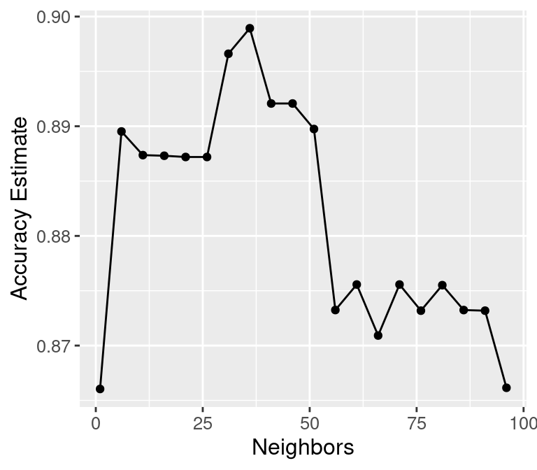
Figure 6.5: Plot of estimated accuracy versus the number of neighbors.
We can also obtain the number of neighbours with the highest accuracy
programmatically by accessing the neighbors variable in the accuracies data
frame where the mean variable is highest.
Note that it is still useful to visualize the results as
we did above since this provides additional information on how the model
performance varies.
## [1] 36Setting the number of neighbors to \(K =\) 36 provides the highest cross-validation accuracy estimate (89.89%). But there is no exact or perfect answer here; any selection from \(K = 30\) and \(60\) would be reasonably justified, as all of these differ in classifier accuracy by a small amount. Remember: the values you see on this plot are estimates of the true accuracy of our classifier. Although the \(K =\) 36 value is higher than the others on this plot, that doesn’t mean the classifier is actually more accurate with this parameter value! Generally, when selecting \(K\) (and other parameters for other predictive models), we are looking for a value where:
- we get roughly optimal accuracy, so that our model will likely be accurate;
- changing the value to a nearby one (e.g., adding or subtracting a small number) doesn’t decrease accuracy too much, so that our choice is reliable in the presence of uncertainty;
- the cost of training the model is not prohibitive (e.g., in our situation, if \(K\) is too large, predicting becomes expensive!).
We know that \(K =\) 36 provides the highest estimated accuracy. Further, Figure 6.5 shows that the estimated accuracy changes by only a small amount if we increase or decrease \(K\) near \(K =\) 36. And finally, \(K =\) 36 does not create a prohibitively expensive computational cost of training. Considering these three points, we would indeed select \(K =\) 36 for the classifier.
6.6.3 Under/Overfitting
To build a bit more intuition, what happens if we keep increasing the number of
neighbors \(K\)? In fact, the accuracy actually starts to decrease!
Let’s specify a much larger range of values of \(K\) to try in the grid
argument of tune_grid. Figure 6.6 shows a plot of estimated accuracy as
we vary \(K\) from 1 to almost the number of observations in the training set.
k_lots <- tibble(neighbors = seq(from = 1, to = 385, by = 10))
knn_results <- workflow() |>
add_recipe(cancer_recipe) |>
add_model(knn_spec) |>
tune_grid(resamples = cancer_vfold, grid = k_lots) |>
collect_metrics()
accuracies_lots <- knn_results |>
filter(.metric == "accuracy")
accuracy_vs_k_lots <- ggplot(accuracies_lots, aes(x = neighbors, y = mean)) +
geom_point() +
geom_line() +
labs(x = "Neighbors", y = "Accuracy Estimate") +
theme(text = element_text(size = 12))
accuracy_vs_k_lots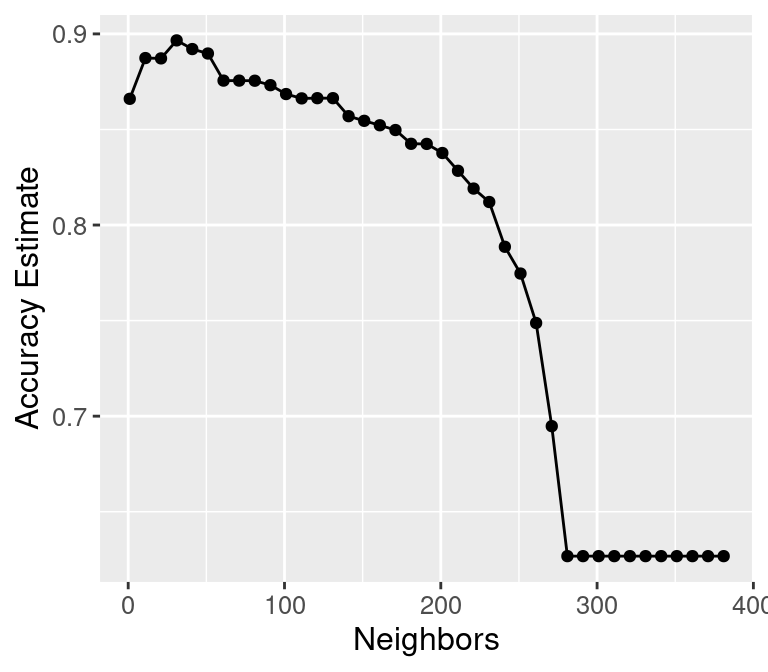
Figure 6.6: Plot of accuracy estimate versus number of neighbors for many K values.
Underfitting: What is actually happening to our classifier that causes this? As we increase the number of neighbors, more and more of the training observations (and those that are farther and farther away from the point) get a “say” in what the class of a new observation is. This causes a sort of “averaging effect” to take place, making the boundary between where our classifier would predict a tumor to be malignant versus benign to smooth out and become simpler. If you take this to the extreme, setting \(K\) to the total training data set size, then the classifier will always predict the same label regardless of what the new observation looks like. In general, if the model isn’t influenced enough by the training data, it is said to underfit the data.
Overfitting: In contrast, when we decrease the number of neighbors, each individual data point has a stronger and stronger vote regarding nearby points. Since the data themselves are noisy, this causes a more “jagged” boundary corresponding to a less simple model. If you take this case to the extreme, setting \(K = 1\), then the classifier is essentially just matching each new observation to its closest neighbor in the training data set. This is just as problematic as the large \(K\) case, because the classifier becomes unreliable on new data: if we had a different training set, the predictions would be completely different. In general, if the model is influenced too much by the training data, it is said to overfit the data.
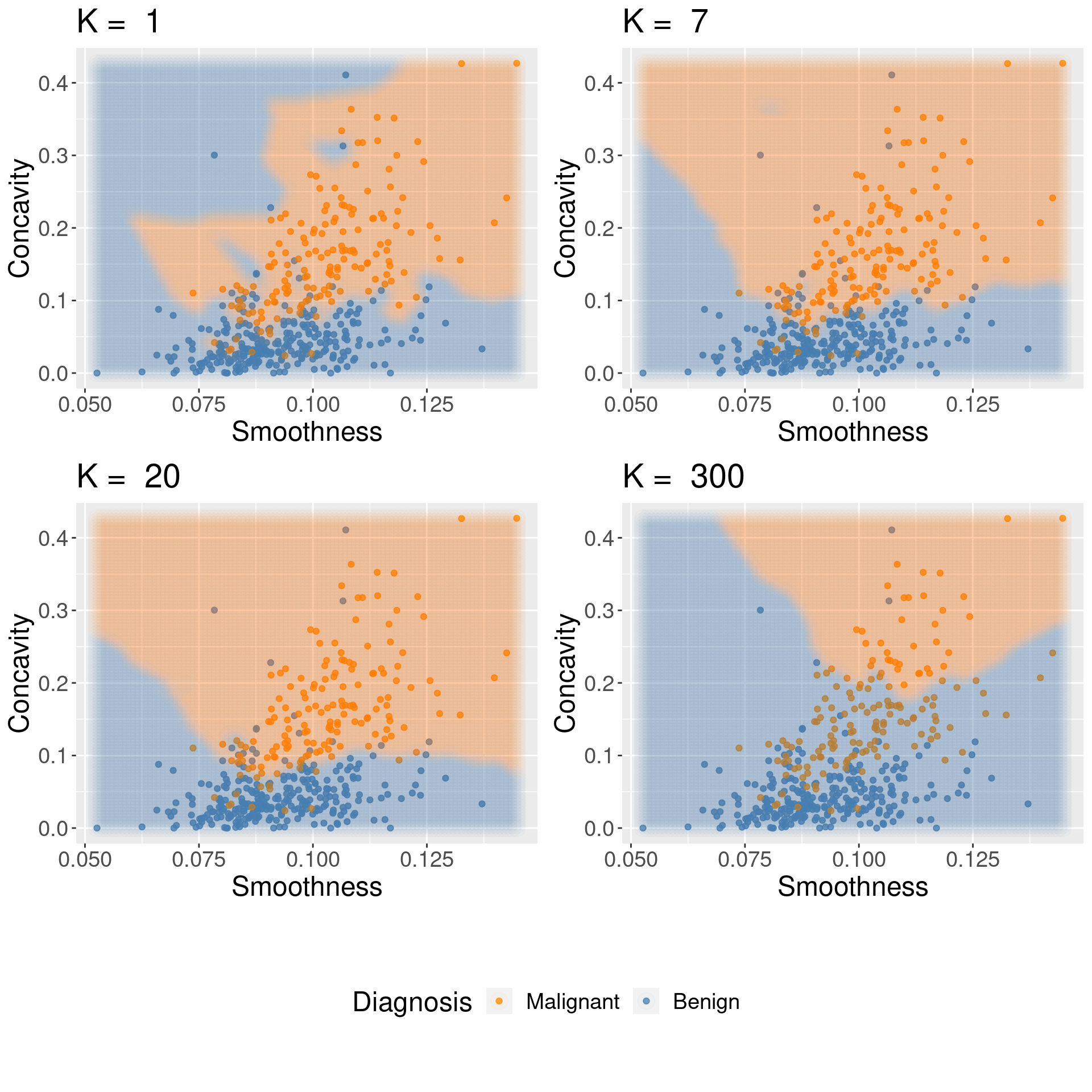
Figure 6.7: Effect of K in overfitting and underfitting.
Both overfitting and underfitting are problematic and will lead to a model that does not generalize well to new data. When fitting a model, we need to strike a balance between the two. You can see these two effects in Figure 6.7, which shows how the classifier changes as we set the number of neighbors \(K\) to 1, 7, 20, and 300.
6.6.4 Evaluating on the test set
Now that we have tuned the K-NN classifier and set \(K =\) 36, we are done building the model and it is time to evaluate the quality of its predictions on the held out test data, as we did earlier in Section 6.5.5. We first need to retrain the K-NN classifier on the entire training data set using the selected number of neighbors.
cancer_recipe <- recipe(Class ~ Smoothness + Concavity, data = cancer_train) |>
step_scale(all_predictors()) |>
step_center(all_predictors())
knn_spec <- nearest_neighbor(weight_func = "rectangular", neighbors = best_k) |>
set_engine("kknn") |>
set_mode("classification")
knn_fit <- workflow() |>
add_recipe(cancer_recipe) |>
add_model(knn_spec) |>
fit(data = cancer_train)
knn_fit## ══ Workflow [trained] ══════════════════════════════════════════════════════════
## Preprocessor: Recipe
## Model: nearest_neighbor()
##
## ── Preprocessor ────────────────────────────────────────────────────────────────
## 2 Recipe Steps
##
## • step_scale()
## • step_center()
##
## ── Model ───────────────────────────────────────────────────────────────────────
##
## Call:
## kknn::train.kknn(formula = ..y ~ ., data = data, ks = min_rows(36, data, 5), kernel = ~"rectangular")
##
## Type of response variable: nominal
## Minimal misclassification: 0.1150235
## Best kernel: rectangular
## Best k: 36Then to make predictions and assess the estimated accuracy of the best model on the test data, we use the
predict and metrics functions as we did earlier in the chapter. We can then pass those predictions to
the precision, recall, and conf_mat functions to assess the estimated precision and recall, and print a confusion matrix.
cancer_test_predictions <- predict(knn_fit, cancer_test) |>
  bind_cols(cancer_test)

cancer_test_predictions |>
metrics(truth = Class, estimate = .pred_class) |>
filter(.metric == "accuracy")## # A tibble: 1 × 3
## .metric .estimator .estimate
## <chr> <chr> <dbl>
## 1 accuracy binary 0.860## # A tibble: 1 × 3
## .metric .estimator .estimate
## <chr> <chr> <dbl>
## 1 precision binary 0.8## # A tibble: 1 × 3
## .metric .estimator .estimate
## <chr> <chr> <dbl>
## 1 recall binary 0.830## Truth
## Prediction Malignant Benign
## Malignant 44 11
## Benign 9 79At first glance, this is a bit surprising: the accuracy of the classifier has only changed a small amount despite tuning the number of neighbors! Our first model with \(K =\) 3 (before we knew how to tune) had an estimated accuracy of 85%, while the tuned model with \(K =\) 36 had an estimated accuracy of 86%. Upon examining Figure 6.5 again to see the cross validation accuracy estimates for a range of neighbors, this result becomes much less surprising. From 1 to around 96 neighbors, the cross validation accuracy estimate varies only by around 3%, with each estimate having a standard error around 1%. Since the cross-validation accuracy estimates the test set accuracy, the fact that the test set accuracy also doesn’t change much is expected. Also note that the \(K =\) 3 model had a precision precision of 77% and recall of 87%, while the tuned model had a precision of 80% and recall of 83%. Given that the recall decreased—remember, in this application, recall is critical to making sure we find all the patients with malignant tumors—the tuned model may actually be less preferred in this setting. In any case, it is important to think critically about the result of tuning. Models tuned to maximize accuracy are not necessarily better for a given application.
6.7 Summary
Classification algorithms use one or more quantitative variables to predict the value of another categorical variable. In particular, the K-nearest neighbors algorithm does this by first finding the \(K\) points in the training data nearest to the new observation, and then returning the majority class vote from those training observations. We can tune and evaluate a classifier by splitting the data randomly into a training and test data set. The training set is used to build the classifier, and we can tune the classifier (e.g., select the number of neighbors in K-NN) by maximizing estimated accuracy via cross-validation. After we have tuned the model we can use the test set to estimate its accuracy. The overall process is summarized in Figure 6.8.
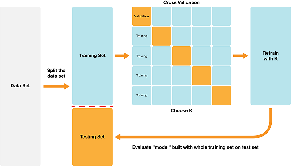
Figure 6.8: Overview of K-NN classification.
The overall workflow for performing K-nearest neighbors classification using tidymodels is as follows:
- Use the
initial_splitfunction to split the data into a training and test set. Set thestrataargument to the class label variable. Put the test set aside for now. - Use the
vfold_cvfunction to split up the training data for cross-validation. - Create a
recipethat specifies the class label and predictors, as well as preprocessing steps for all variables. Pass the training data as thedataargument of the recipe. - Create a
nearest_neighborsmodel specification, withneighbors = tune(). - Add the recipe and model specification to a
workflow(), and use thetune_gridfunction on the train/validation splits to estimate the classifier accuracy for a range of \(K\) values. - Pick a value of \(K\) that yields a high accuracy estimate that doesn’t change much if you change \(K\) to a nearby value.
- Make a new model specification for the best parameter value (i.e., \(K\)), and retrain the classifier using the
fitfunction. - Evaluate the estimated accuracy of the classifier on the test set using the
predictfunction.
In these last two chapters, we focused on the K-nearest neighbors algorithm, but there are many other methods we could have used to predict a categorical label. All algorithms have their strengths and weaknesses, and we summarize these for the K-NN here.
Strengths: K-nearest neighbors classification
- is a simple, intuitive algorithm,
- requires few assumptions about what the data must look like, and
- works for binary (two-class) and multi-class (more than 2 classes) classification problems.
Weaknesses: K-nearest neighbors classification
- becomes very slow as the training data gets larger,
- may not perform well with a large number of predictors, and
- may not perform well when classes are imbalanced.
6.8 Predictor variable selection
Note: This section is not required reading for the remainder of the textbook. It is included for those readers interested in learning how irrelevant variables can influence the performance of a classifier, and how to pick a subset of useful variables to include as predictors.
Another potentially important part of tuning your classifier is to choose which variables from your data will be treated as predictor variables. Technically, you can choose anything from using a single predictor variable to using every variable in your data; the K-nearest neighbors algorithm accepts any number of predictors. However, it is not the case that using more predictors always yields better predictions! In fact, sometimes including irrelevant predictors can actually negatively affect classifier performance.
6.8.1 The effect of irrelevant predictors
Let’s take a look at an example where K-nearest neighbors performs
worse when given more predictors to work with. In this example, we modified
the breast cancer data to have only the Smoothness, Concavity, and
Perimeter variables from the original data. Then, we added irrelevant
variables that we created ourselves using a random number generator.
The irrelevant variables each take a value of 0 or 1 with equal probability for each observation, regardless
of what the value Class variable takes. In other words, the irrelevant variables have
no meaningful relationship with the Class variable.
## # A tibble: 569 × 6
## Class Smoothness Concavity Perimeter Irrelevant1 Irrelevant2
## <fct> <dbl> <dbl> <dbl> <dbl> <dbl>
## 1 Malignant 0.118 0.300 123. 1 0
## 2 Malignant 0.0847 0.0869 133. 0 0
## 3 Malignant 0.110 0.197 130 0 0
## 4 Malignant 0.142 0.241 77.6 0 1
## 5 Malignant 0.100 0.198 135. 0 0
## 6 Malignant 0.128 0.158 82.6 1 0
## 7 Malignant 0.0946 0.113 120. 0 1
## 8 Malignant 0.119 0.0937 90.2 1 0
## 9 Malignant 0.127 0.186 87.5 0 0
## 10 Malignant 0.119 0.227 84.0 1 1
## # ℹ 559 more rowsNext, we build a sequence of K-NN classifiers that include Smoothness,
Concavity, and Perimeter as predictor variables, but also increasingly many irrelevant
variables. In particular, we create 6 data sets with 0, 5, 10, 15, 20, and 40 irrelevant predictors.
Then we build a model, tuned via 5-fold cross-validation, for each data set.
Figure 6.9 shows
the estimated cross-validation accuracy versus the number of irrelevant predictors. As
we add more irrelevant predictor variables, the estimated accuracy of our
classifier decreases. This is because the irrelevant variables add a random
amount to the distance between each pair of observations; the more irrelevant
variables there are, the more (random) influence they have, and the more they
corrupt the set of nearest neighbors that vote on the class of the new
observation to predict.
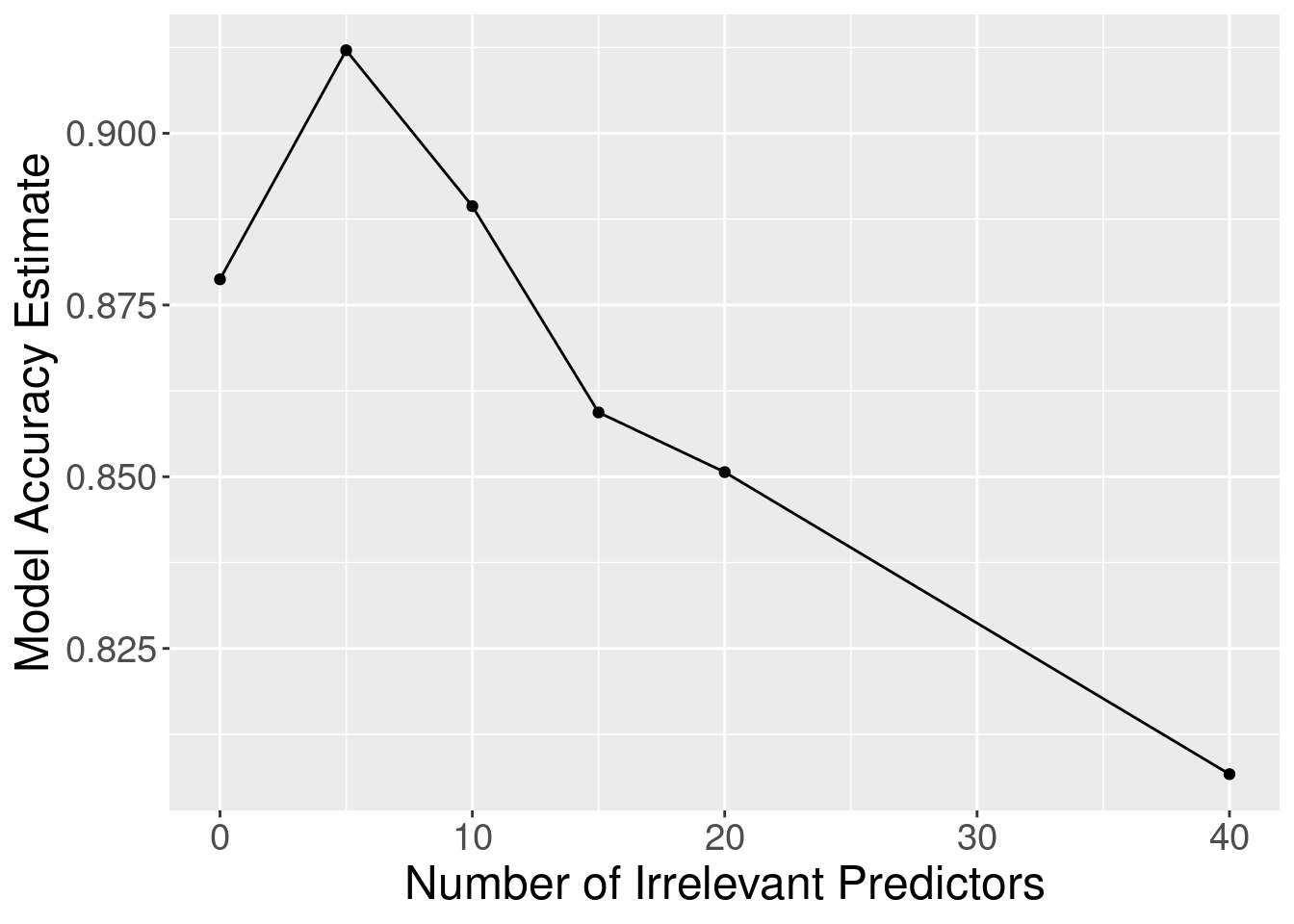
Figure 6.9: Effect of inclusion of irrelevant predictors.
Although the accuracy decreases as expected, one surprising thing about Figure 6.9 is that it shows that the method still outperforms the baseline majority classifier (with about 63% accuracy) even with 40 irrelevant variables. How could that be? Figure 6.10 provides the answer: the tuning procedure for the K-nearest neighbors classifier combats the extra randomness from the irrelevant variables by increasing the number of neighbors. Of course, because of all the extra noise in the data from the irrelevant variables, the number of neighbors does not increase smoothly; but the general trend is increasing. Figure 6.11 corroborates this evidence; if we fix the number of neighbors to \(K=3\), the accuracy falls off more quickly.
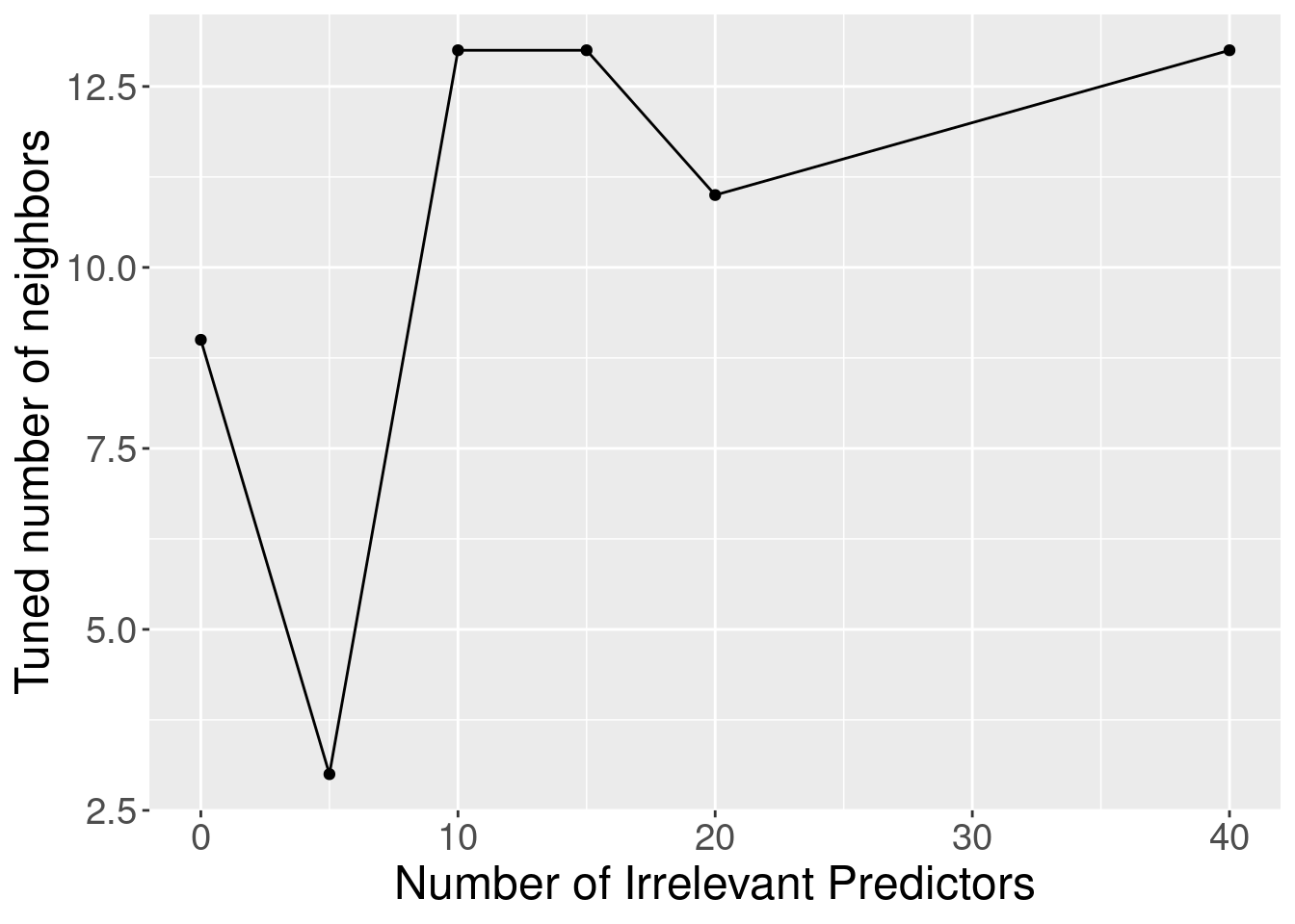
Figure 6.10: Tuned number of neighbors for varying number of irrelevant predictors.
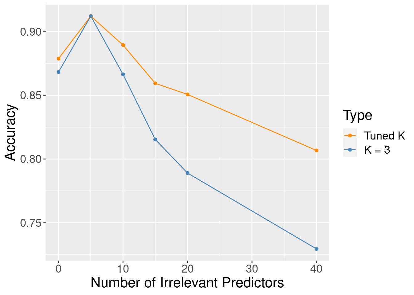
Figure 6.11: Accuracy versus number of irrelevant predictors for tuned and untuned number of neighbors.
6.8.2 Finding a good subset of predictors
So then, if it is not ideal to use all of our variables as predictors without consideration, how
do we choose which variables we should use? A simple method is to rely on your scientific understanding
of the data to tell you which variables are not likely to be useful predictors. For example, in the cancer
data that we have been studying, the ID variable is just a unique identifier for the observation.
As it is not related to any measured property of the cells, the ID variable should therefore not be used
as a predictor. That is, of course, a very clear-cut case. But the decision for the remaining variables
is less obvious, as all seem like reasonable candidates. It
is not clear which subset of them will create the best classifier. One could use visualizations and
other exploratory analyses to try to help understand which variables are potentially relevant, but
this process is both time-consuming and error-prone when there are many variables to consider.
Therefore we need a more systematic and programmatic way of choosing variables.
This is a very difficult problem to solve in
general, and there are a number of methods that have been developed that apply
in particular cases of interest. Here we will discuss two basic
selection methods as an introduction to the topic. See the additional resources at the end of
this chapter to find out where you can learn more about variable selection, including more advanced methods.
The first idea you might think of for a systematic way to select predictors is to try all possible subsets of predictors and then pick the set that results in the “best” classifier. This procedure is indeed a well-known variable selection method referred to as best subset selection (Beale, Kendall, and Mann 1967; Hocking and Leslie 1967). In particular, you
- create a separate model for every possible subset of predictors,
- tune each one using cross-validation, and
- pick the subset of predictors that gives you the highest cross-validation accuracy.
Best subset selection is applicable to any classification method (K-NN or otherwise). However, it becomes very slow when you have even a moderate number of predictors to choose from (say, around 10). This is because the number of possible predictor subsets grows very quickly with the number of predictors, and you have to train the model (itself a slow process!) for each one. For example, if we have 2 predictors—let’s call them A and B—then we have 3 variable sets to try: A alone, B alone, and finally A and B together. If we have 3 predictors—A, B, and C—then we have 7 to try: A, B, C, AB, BC, AC, and ABC. In general, the number of models we have to train for \(m\) predictors is \(2^m-1\); in other words, when we get to 10 predictors we have over one thousand models to train, and at 20 predictors we have over one million models to train! So although it is a simple method, best subset selection is usually too computationally expensive to use in practice.
Another idea is to iteratively build up a model by adding one predictor variable at a time. This method—known as forward selection (Eforymson 1966; Draper and Smith 1966)—is also widely applicable and fairly straightforward. It involves the following steps:
- Start with a model having no predictors.
- Run the following 3 steps until you run out of predictors:
- For each unused predictor, add it to the model to form a candidate model.
- Tune all of the candidate models.
- Update the model to be the candidate model with the highest cross-validation accuracy.
- Select the model that provides the best trade-off between accuracy and simplicity.
Say you have \(m\) total predictors to work with. In the first iteration, you have to make \(m\) candidate models, each with 1 predictor. Then in the second iteration, you have to make \(m-1\) candidate models, each with 2 predictors (the one you chose before and a new one). This pattern continues for as many iterations as you want. If you run the method all the way until you run out of predictors to choose, you will end up training \(\frac{1}{2}m(m+1)\) separate models. This is a big improvement from the \(2^m-1\) models that best subset selection requires you to train! For example, while best subset selection requires training over 1000 candidate models with 10 predictors, forward selection requires training only 55 candidate models. Therefore we will continue the rest of this section using forward selection.
Note: One word of caution before we move on. Every additional model that you train increases the likelihood that you will get unlucky and stumble on a model that has a high cross-validation accuracy estimate, but a low true accuracy on the test data and other future observations. Since forward selection involves training a lot of models, you run a fairly high risk of this happening. To keep this risk low, only use forward selection when you have a large amount of data and a relatively small total number of predictors. More advanced methods do not suffer from this problem as much; see the additional resources at the end of this chapter for where to learn more about advanced predictor selection methods.
6.8.3 Forward selection in R
We now turn to implementing forward selection in R.
Unfortunately there is no built-in way to do this using the tidymodels framework,
so we will have to code it ourselves. First we will use the select function to extract a smaller set of predictors
to work with in this illustrative example—Smoothness, Concavity, Perimeter, Irrelevant1, Irrelevant2, and Irrelevant3—as
well as the Class variable as the label. We will also extract the column names for the full set of predictors.
cancer_subset <- cancer_irrelevant |>
select(Class,
Smoothness,
Concavity,
Perimeter,
Irrelevant1,
Irrelevant2,
Irrelevant3)
names <- colnames(cancer_subset |> select(-Class))
cancer_subset## # A tibble: 569 × 7
## Class Smoothness Concavity Perimeter Irrelevant1 Irrelevant2 Irrelevant3
## <fct> <dbl> <dbl> <dbl> <dbl> <dbl> <dbl>
## 1 Malignant 0.118 0.300 123. 1 0 1
## 2 Malignant 0.0847 0.0869 133. 0 0 0
## 3 Malignant 0.110 0.197 130 0 0 0
## 4 Malignant 0.142 0.241 77.6 0 1 0
## 5 Malignant 0.100 0.198 135. 0 0 0
## 6 Malignant 0.128 0.158 82.6 1 0 1
## 7 Malignant 0.0946 0.113 120. 0 1 1
## 8 Malignant 0.119 0.0937 90.2 1 0 0
## 9 Malignant 0.127 0.186 87.5 0 0 1
## 10 Malignant 0.119 0.227 84.0 1 1 0
## # ℹ 559 more rowsThe key idea of the forward selection code is to use the paste function (which concatenates strings
separated by spaces) to create a model formula for each subset of predictors for which we want to build a model.
The collapse argument tells paste what to put between the items in the list;
to make a formula, we need to put a + symbol between each variable.
As an example, let’s make a model formula for all the predictors,
which should output something like
Class ~ Smoothness + Concavity + Perimeter + Irrelevant1 + Irrelevant2 + Irrelevant3:
## [1] "Class ~ Smoothness+Concavity+Perimeter+Irrelevant1+Irrelevant2+Irrelevant3"Finally, we need to write some code that performs the task of sequentially
finding the best predictor to add to the model.
If you recall the end of the wrangling chapter, we mentioned
that sometimes one needs more flexible forms of iteration than what
we have used earlier, and in these cases one typically resorts to
a for loop; see the chapter on iteration in R for Data Science (Wickham and Grolemund 2016).
Here we will use two for loops:
one over increasing predictor set sizes
(where you see for (i in 1:length(names)) below),
and another to check which predictor to add in each round (where you see for (j in 1:length(names)) below).
For each set of predictors to try, we construct a model formula,
pass it into a recipe, build a workflow that tunes
a K-NN classifier using 5-fold cross-validation,
and finally records the estimated accuracy.
# create an empty tibble to store the results
accuracies <- tibble(size = integer(),
model_string = character(),
accuracy = numeric())
# create a model specification
knn_spec <- nearest_neighbor(weight_func = "rectangular",
                             neighbors = tune()) |>
  set_engine("kknn") |>
  set_mode("classification")
# create a 5-fold cross-validation object
cancer_vfold <- vfold_cv(cancer_subset, v = 5, strata = Class)
# store the total number of predictors
n_total <- length(names)
# stores selected predictors
selected <- c()
# for every size from 1 to the total number of predictors
for (i in 1:n_total) {
# for every predictor still not added yet
accs <- list()
models <- list()
for (j in 1:length(names)) {
# create a model string for this combination of predictors
preds_new <- c(selected, names[[j]])
model_string <- paste("Class", "~", paste(preds_new, collapse="+"))
# create a recipe from the model string
cancer_recipe <- recipe(as.formula(model_string),
data = cancer_subset) |>
step_scale(all_predictors()) |>
step_center(all_predictors())
# tune the K-NN classifier with these predictors,
# and collect the accuracy for the best K
acc <- workflow() |>
add_recipe(cancer_recipe) |>
add_model(knn_spec) |>
tune_grid(resamples = cancer_vfold, grid = 10) |>
collect_metrics() |>
filter(.metric == "accuracy") |>
summarize(mx = max(mean))
acc <- acc$mx |> unlist()
# add this result to the dataframe
accs[[j]] <- acc
models[[j]] <- model_string
}
jstar <- which.max(unlist(accs))
accuracies <- accuracies |>
add_row(size = i,
model_string = models[[jstar]],
accuracy = accs[[jstar]])
selected <- c(selected, names[[jstar]])
names <- names[-jstar]
}
accuracies## # A tibble: 6 × 3
## size model_string accuracy
## <int> <chr> <dbl>
## 1 1 Class ~ Perimeter 0.896
## 2 2 Class ~ Perimeter+Concavity 0.916
## 3 3 Class ~ Perimeter+Concavity+Smoothness 0.931
## 4 4 Class ~ Perimeter+Concavity+Smoothness+Irrelevant1 0.928
## 5 5 Class ~ Perimeter+Concavity+Smoothness+Irrelevant1+Irrelevant3 0.924
## 6 6 Class ~ Perimeter+Concavity+Smoothness+Irrelevant1+Irrelevant3… 0.902Interesting! The forward selection procedure first added the three meaningful variables Perimeter,
Concavity, and Smoothness, followed by the irrelevant variables. Figure 6.12
visualizes the accuracy versus the number of predictors in the model. You can see that
as meaningful predictors are added, the estimated accuracy increases substantially; and as you add irrelevant
variables, the accuracy either exhibits small fluctuations or decreases as the model attempts to tune the number
of neighbors to account for the extra noise. In order to pick the right model from the sequence, you have
to balance high accuracy and model simplicity (i.e., having fewer predictors and a lower chance of overfitting). The
way to find that balance is to look for the elbow
in Figure 6.12, i.e., the place on the plot where the accuracy stops increasing dramatically and
levels off or begins to decrease. The elbow in Figure 6.12 appears to occur at the model with
3 predictors; after that point the accuracy levels off. So here the right trade-off of accuracy and number of predictors
occurs with 3 variables: Class ~ Perimeter + Concavity + Smoothness. In other words, we have successfully removed irrelevant
predictors from the model! It is always worth remembering, however, that what cross-validation gives you
is an estimate of the true accuracy; you have to use your judgement when looking at this plot to decide
where the elbow occurs, and whether adding a variable provides a meaningful increase in accuracy.
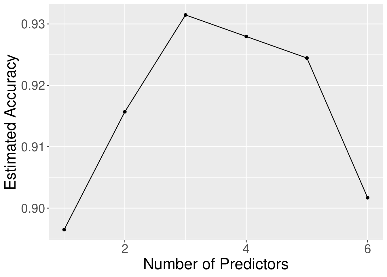
Figure 6.12: Estimated accuracy versus the number of predictors for the sequence of models built using forward selection.
Note: Since the choice of which variables to include as predictors is part of tuning your classifier, you cannot use your test data for this process!
6.9 Exercises
Practice exercises for the material covered in this chapter can be found in the accompanying worksheets repository in the “Classification II: evaluation and tuning” row. You can launch an interactive version of the worksheet in your browser by clicking the “launch binder” button. You can also preview a non-interactive version of the worksheet by clicking “view worksheet.” If you instead decide to download the worksheet and run it on your own machine, make sure to follow the instructions for computer setup found in Chapter 13. This will ensure that the automated feedback and guidance that the worksheets provide will function as intended.
6.10 Additional resources
- The
tidymodelswebsite is an excellent reference for more details on, and advanced usage of, the functions and packages in the past two chapters. Aside from that, it also has a nice beginner’s tutorial and an extensive list of more advanced examples that you can use to continue learning beyond the scope of this book. It’s worth noting that thetidymodelspackage does a lot more than just classification, and so the examples on the website similarly go beyond classification as well. In the next two chapters, you’ll learn about another kind of predictive modeling setting, so it might be worth visiting the website only after reading through those chapters. - An Introduction to Statistical Learning (James et al. 2013) provides a great next stop in the process of learning about classification. Chapter 4 discusses additional basic techniques for classification that we do not cover, such as logistic regression, linear discriminant analysis, and naive Bayes. Chapter 5 goes into much more detail about cross-validation. Chapters 8 and 9 cover decision trees and support vector machines, two very popular but more advanced classification methods. Finally, Chapter 6 covers a number of methods for selecting predictor variables. Note that while this book is still a very accessible introductory text, it requires a bit more mathematical background than we require.