 Data Science
Chapter 3 Cleaning and wrangling data
3.1 Overview
This chapter is centered around defining tidy data—a data format that is suitable for analysis—and the tools needed to transform raw data into this format. This will be presented in the context of a real-world data science application, providing more practice working through a whole case study.
3.2 Chapter learning objectives
By the end of the chapter, readers will be able to do the following:
- Define the term “tidy data”.
- Discuss the advantages of storing data in a tidy data format.
- Define what vectors, lists, and data frames are in R, and describe how they relate to each other.
- Describe the common types of data in R and their uses.
- Use the following functions for their intended data wrangling tasks:
cpivot_longerpivot_widerseparateselectfiltermutatesummarizemapgroup_byacrossrowwise
- Use the following operators for their intended data wrangling tasks:
==,!=,<,<=,>, and>=%in%!,&, and||>and%>%
3.3 Data frames, vectors, and lists
In Chapters 1 and 2, data frames were the focus: we learned how to import data into R as a data frame, and perform basic operations on data frames in R. In the remainder of this book, this pattern continues. The vast majority of tools we use will require that data are represented as a data frame in R. Therefore, in this section, we will dig more deeply into what data frames are and how they are represented in R. This knowledge will be helpful in effectively utilizing these objects in our data analyses.
3.3.1 What is a data frame?
A data frame is a table-like structure for storing data in R. Data frames are important to learn about because most data that you will encounter in practice can be naturally stored as a table. In order to define data frames precisely, we need to introduce a few technical terms:
- variable: a characteristic, number, or quantity that can be measured.
- observation: all of the measurements for a given entity.
- value: a single measurement of a single variable for a given entity.
Given these definitions, a data frame is a tabular data structure in R that is designed to store observations, variables, and their values. Most commonly, each column in a data frame corresponds to a variable, and each row corresponds to an observation. For example, Figure 3.1 displays a data set of city populations. Here, the variables are “region, year, population”; each of these are properties that can be collected or measured. The first observation is “Toronto, 2016, 2235145”; these are the values that the three variables take for the first entity in the data set. There are 13 entities in the data set in total, corresponding to the 13 rows in Figure 3.1.
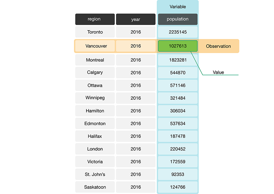
Figure 3.1: A data frame storing data regarding the population of various regions in Canada. In this example data frame, the row that corresponds to the observation for the city of Vancouver is colored yellow, and the column that corresponds to the population variable is colored blue.
R stores the columns of a data frame as either
lists or vectors. For example, the data frame in Figure
3.2 has three vectors whose names are region, year and
population. The next two sections will explain what lists and vectors are.
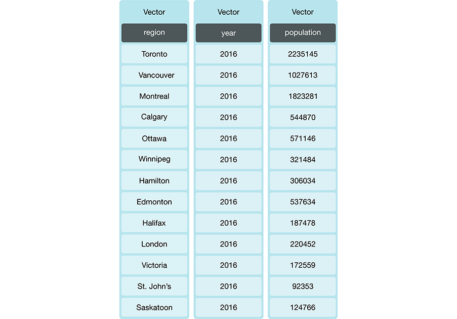
Figure 3.2: Data frame with three vectors.
3.3.2 What is a vector?
In R, vectors are objects that can contain one or more elements. The vector
elements are ordered, and they must all be of the same data type;
R has several different basic data types, as shown in Table 3.1.
Figure 3.3 provides an example of a vector where all of the elements are
of character type.
You can create vectors in R using the c function (c stands for “concatenate”). For
example, to create the vector region as shown in Figure
3.3, you would write:
## [1] "Toronto" "Montreal" "Vancouver" "Calgary" "Ottawa"Note: Technically, these objects are called “atomic vectors.” In this book we have chosen to call them “vectors,” which is how they are most commonly referred to in the R community. To be totally precise, “vector” is an umbrella term that encompasses both atomic vector and list objects in R. But this creates a confusing situation where the term “vector” could mean “atomic vector” or “the umbrella term for atomic vector and list,” depending on context. Very confusing indeed! So to keep things simple, in this book we always use the term “vector” to refer to “atomic vector.” We encourage readers who are enthusiastic to learn more to read the Vectors chapter of Advanced R (Wickham 2019).

Figure 3.3: Example of a vector whose type is character.
| Data type | Abbreviation | Description | Example |
|---|---|---|---|
| character | chr | letters or numbers surrounded by quotes | “1” , “Hello world!” |
| double | dbl | numbers with decimals values | 1.2333 |
| integer | int | numbers that do not contain decimals | 1L, 20L (where “L” tells R to store as an integer) |
| logical | lgl | either true or false | TRUE, FALSE |
| factor | fct | used to represent data with a limited number of values (usually categories) | a color variable with levels red, green and orange |
It is important in R to make sure you represent your data with the correct type.
Many of the tidyverse functions we use in this book treat
the various data types differently. You should use integers and double types
(which both fall under the “numeric” umbrella type) to represent numbers and perform
arithmetic. Doubles are more common than integers in R, though; for instance, a double data type is the
default when you create a vector of numbers using c(), and when you read in
whole numbers via read_csv. Characters are used to represent data that should
be thought of as “text”, such as words, names, paths, URLs, and more. Factors help us
encode variables that represent categories; a factor variable takes one of a discrete
set of values known as levels (one for each category). The levels can be ordered or unordered. Even though
factors can sometimes look like characters, they are not used to represent
text, words, names, and paths in the way that characters are; in fact, R
internally stores factors using integers! There are other basic data types in R, such as raw
and complex, but we do not use these in this textbook.
3.3.3 What is a list?
Lists are also objects in R that have multiple, ordered elements. Vectors and lists differ by the requirement of element type consistency. All elements within a single vector must be of the same type (e.g., all elements are characters), whereas elements within a single list can be of different types (e.g., characters, integers, logicals, and even other lists). See Figure 3.4.
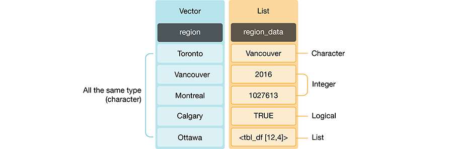
Figure 3.4: A vector versus a list.
3.3.4 What does this have to do with data frames?
A data frame is really a special kind of list that follows two rules:
- Each element itself must either be a vector or a list.
- Each element (vector or list) must have the same length.
Not all columns in a data frame need to be of the same type. Figure 3.5 shows a data frame where the columns are vectors of different types. But remember: because the columns in this example are vectors, the elements must be the same data type within each column. On the other hand, if our data frame had list columns, there would be no such requirement. It is generally much more common to use vector columns, though, as the values for a single variable are usually all of the same type.
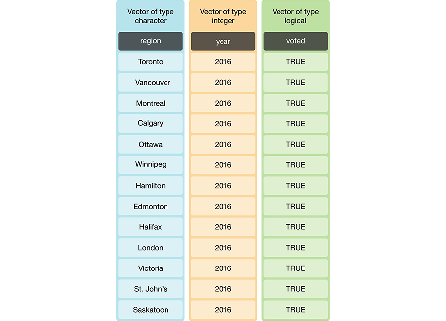
Figure 3.5: Data frame and vector types.
Data frames are actually included in R itself, without the need for any additional packages. However, the
tidyverse functions that we use
throughout this book all work with a special kind of data frame called a tibble. Tibbles have some additional
features and benefits over built-in data frames in R. These include the
ability to add useful attributes (such as grouping, which we will discuss later)
and more predictable type preservation when subsetting.
Because a tibble is just a data frame with some added features,
we will collectively refer to both built-in R data frames and
tibbles as data frames in this book.
Note: You can use the function
classon a data object to assess whether a data frame is a built-in R data frame or a tibble. If the data object is a data frame,classwill return"data.frame". If the data object is a tibble it will return"tbl_df" "tbl" "data.frame". You can easily convert built-in R data frames to tibbles using thetidyverseas_tibblefunction. For example we can check the class of the Canadian languages data set,can_lang, we worked with in the previous chapters and we see it is a tibble.## [1] "spec_tbl_df" "tbl_df" "tbl" "data.frame"
Vectors, data frames and lists are basic types of data structure in R, which are core to most data analyses. We summarize them in Table 3.2. There are several other data structures in the R programming language (e.g., matrices), but these are beyond the scope of this book.
| Data Structure | Description |
|---|---|
| vector | An ordered collection of one, or more, values of the same data type. |
| list | An ordered collection of one, or more, values of possibly different data types. |
| data frame | A list of either vectors or lists of the same length, with column names. We typically use a data frame to represent a data set. |
3.4 Tidy data
There are many ways a tabular data set can be organized. This chapter will focus on introducing the tidy data format of organization and how to make your raw (and likely messy) data tidy. A tidy data frame satisfies the following three criteria (Wickham 2014):
- each row is a single observation,
- each column is a single variable, and
- each value is a single cell (i.e., its entry in the data frame is not shared with another value).
Figure 3.6 demonstrates a tidy data set that satisfies these three criteria.
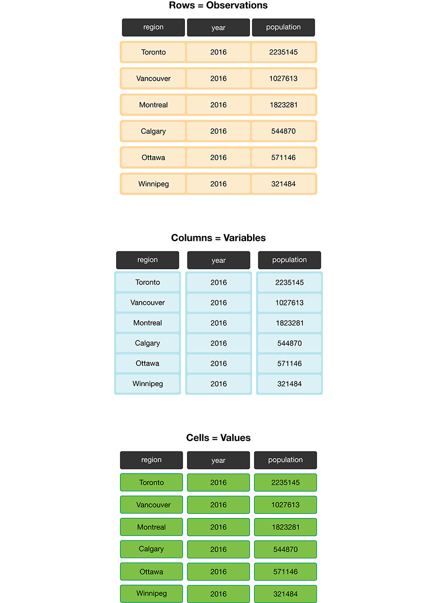
Figure 3.6: Tidy data satisfies three criteria.
There are many good reasons for making sure your data are tidy as a first step in your analysis.
The most important is that it is a single, consistent format that nearly every function
in the tidyverse recognizes. No matter what the variables and observations
in your data represent, as long as the data frame
is tidy, you can manipulate it, plot it, and analyze it using the same tools.
If your data is not tidy, you will have to write special bespoke code
in your analysis that will not only be error-prone, but hard for others to understand.
Beyond making your analysis more accessible to others and less error-prone, tidy data
is also typically easy for humans to interpret. Given these benefits,
it is well worth spending the time to get your data into a tidy format
upfront. Fortunately, there are many well-designed tidyverse data
cleaning/wrangling tools to help you easily tidy your data. Let’s explore them
below!
Note: Is there only one shape for tidy data for a given data set? Not necessarily! It depends on the statistical question you are asking and what the variables are for that question. For tidy data, each variable should be its own column. So, just as it’s essential to match your statistical question with the appropriate data analysis tool, it’s important to match your statistical question with the appropriate variables and ensure they are represented as individual columns to make the data tidy.
3.4.1 Tidying up: going from wide to long using pivot_longer
One task that is commonly performed to get data into a tidy format is to combine values that are stored in separate columns, but are really part of the same variable, into one. Data is often stored this way because this format is sometimes more intuitive for human readability and understanding, and humans create data sets. In Figure 3.7, the table on the left is in an untidy, “wide” format because the year values (2006, 2011, 2016) are stored as column names. And as a consequence, the values for population for the various cities over these years are also split across several columns.
For humans, this table is easy to read, which is why you will often find data
stored in this wide format. However, this format is difficult to work with
when performing data visualization or statistical analysis using R. For
example, if we wanted to find the latest year it would be challenging because
the year values are stored as column names instead of as values in a single
column. So before we could apply a function to find the latest year (for
example, by using max), we would have to first extract the column names
to get them as a vector and then apply a function to extract the latest year.
The problem only gets worse if you would like to find the value for the
population for a given region for the latest year. Both of these tasks are
greatly simplified once the data is tidied.
Another problem with data in this format is that we don’t know what the numbers under each year actually represent. Do those numbers represent population size? Land area? It’s not clear. To solve both of these problems, we can reshape this data set to a tidy data format by creating a column called “year” and a column called “population.” This transformation—which makes the data “longer”—is shown as the right table in Figure 3.7.
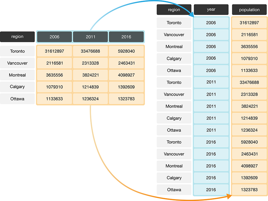
Figure 3.7: Pivoting data from a wide to long data format.
We can achieve this effect in R using the pivot_longer function from the tidyverse package.
The pivot_longer function combines columns,
and is usually used during tidying data
when we need to make the data frame longer and narrower.
To learn how to use pivot_longer, we will work through an example with the
region_lang_top5_cities_wide.csv data set. This data set contains the
counts of how many Canadians cited each language as their mother tongue for five
major Canadian cities (Toronto, Montréal, Vancouver, Calgary, and Edmonton) from
the 2016 Canadian census.
To get started,
we will load the tidyverse package and use read_csv to load the (untidy) data.
## # A tibble: 214 × 7
##    category                 language Toronto Montréal Vancouver Calgary Edmonton
##    <chr>                    <chr>      <dbl>    <dbl>     <dbl>   <dbl>    <dbl>
##  1 Aboriginal languages     Aborigi…      80       30        70      20       25
##  2 Non-Official & Non-Abor… Afrikaa…     985       90      1435     960      575
##  3 Non-Official & Non-Abor… Afro-As…     360      240        45      45       65
##  4 Non-Official & Non-Abor… Akan (T…    8485     1015       400     705      885
##  5 Non-Official & Non-Abor… Albanian   13260     2450      1090    1365      770
##  6 Aboriginal languages     Algonqu…       5        5         0       0        0
##  7 Aboriginal languages     Algonqu…       5       30         5       5        0
##  8 Non-Official & Non-Abor… America…     470       50       265     100      180
##  9 Non-Official & Non-Abor… Amharic     7460      665      1140    4075     2515
## 10 Non-Official & Non-Abor… Arabic     85175   151955     14320   18965    17525
## # ℹ 204 more rows
What is wrong with the untidy format above?
The table on the left in Figure 3.8
represents the data in the “wide” (messy) format.
From a data analysis perspective, this format is not ideal because the values of
the variable region (Toronto, Montréal, Vancouver, Calgary, and Edmonton)
are stored as column names. Thus they
are not easily accessible to the data analysis functions we will apply
to our data set. Additionally, the mother tongue variable values are
spread across multiple columns, which will prevent us from doing any desired
visualization or statistical tasks until we combine them into one column. For
instance, suppose we want to know the languages with the highest number of
Canadians reporting it as their mother tongue among all five regions. This
question would be tough to answer with the data in its current format.
We could find the answer with the data in this format,
though it would be much easier to answer if we tidy our
data first. If mother tongue were instead stored as one column,
as shown in the tidy data on the right in
Figure 3.8,
we could simply use the max function in one line of code
to get the maximum value.
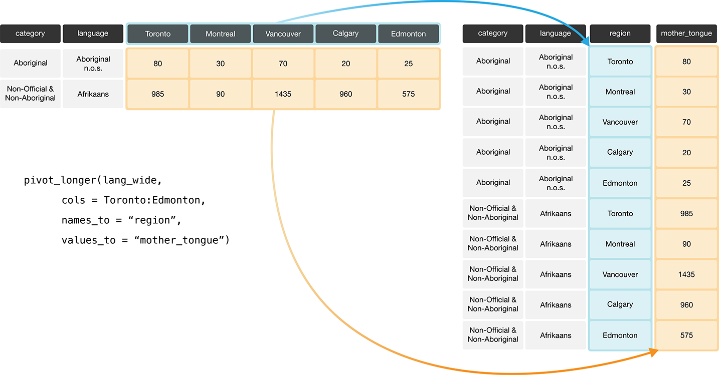
Figure 3.8: Going from wide to long with the pivot_longer function.
Figure 3.9 details the arguments that we need to specify
in the pivot_longer function to accomplish this data transformation.
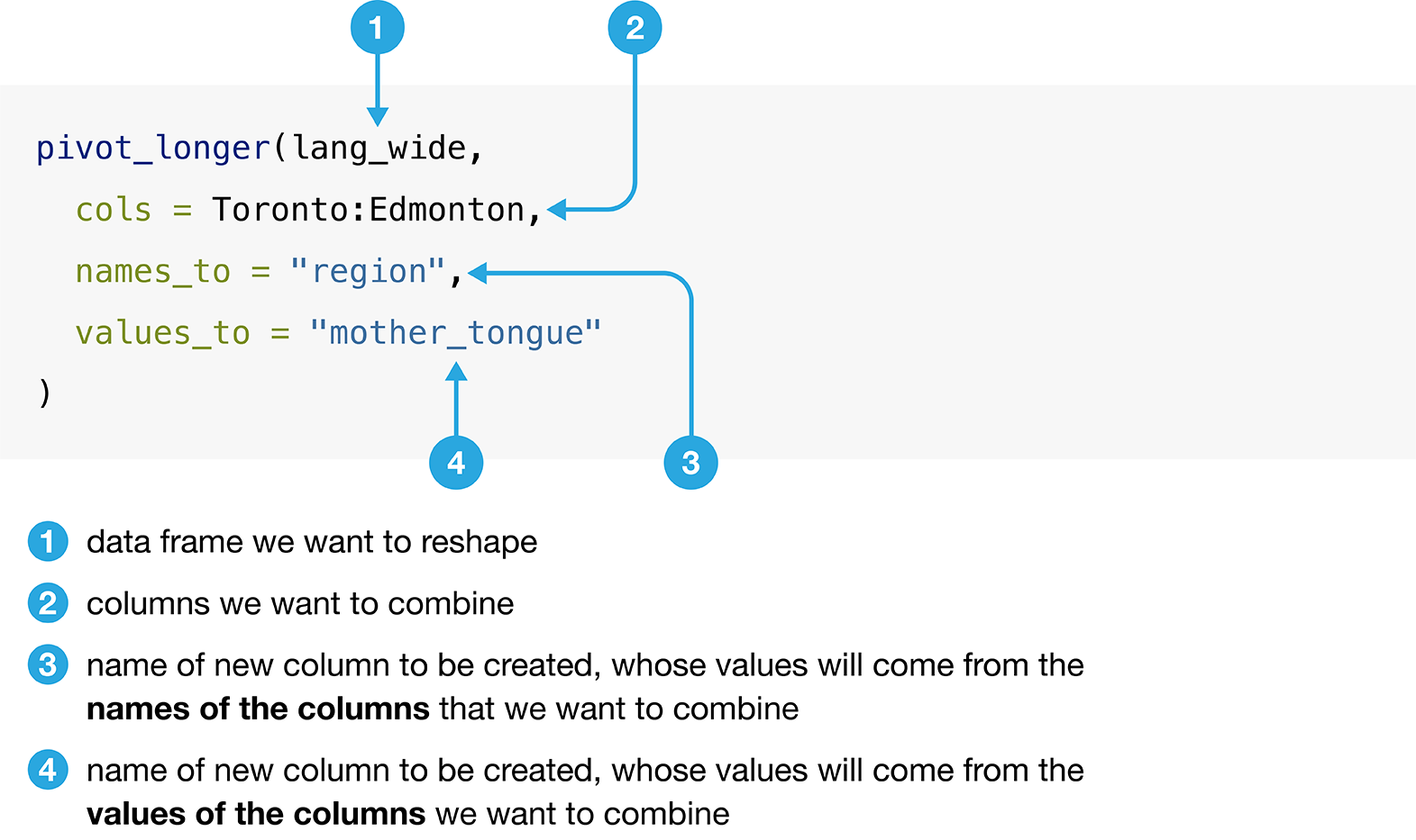
Figure 3.9: Syntax for the pivot_longer function.
We use pivot_longer to combine the Toronto, Montréal,
Vancouver, Calgary, and Edmonton columns into a single column called region,
and create a column called mother_tongue that contains the count of how many
Canadians report each language as their mother tongue for each metropolitan
area. We use a colon : between Toronto and Edmonton to tell R to select all
the columns between Toronto and Edmonton:
lang_mother_tidy <- pivot_longer(lang_wide,
  cols = Toronto:Edmonton,
  names_to = "region",
  values_to = "mother_tongue"
)

lang_mother_tidy
## # A tibble: 1,070 × 4
## category language region mother_tongue
## <chr> <chr> <chr> <dbl>
## 1 Aboriginal languages Aboriginal lang… Toron… 80
## 2 Aboriginal languages Aboriginal lang… Montr… 30
## 3 Aboriginal languages Aboriginal lang… Vanco… 70
## 4 Aboriginal languages Aboriginal lang… Calga… 20
## 5 Aboriginal languages Aboriginal lang… Edmon… 25
## 6 Non-Official & Non-Aboriginal languages Afrikaans Toron… 985
## 7 Non-Official & Non-Aboriginal languages Afrikaans Montr… 90
## 8 Non-Official & Non-Aboriginal languages Afrikaans Vanco… 1435
## 9 Non-Official & Non-Aboriginal languages Afrikaans Calga… 960
## 10 Non-Official & Non-Aboriginal languages Afrikaans Edmon… 575
## # ℹ 1,060 more rowsNote: In the code above, the call to the
pivot_longerfunction is split across several lines. This is allowed in certain cases; for example, when calling a function as above, as long as the line ends with a comma,R knows to keep reading on the next line. Splitting long lines like this across multiple lines is encouraged as it helps significantly with code readability. Generally speaking, you should limit each line of code to about 80 characters.
The data above is now tidy because all three criteria for tidy data have now been met:
- All the variables (
category,language,regionandmother_tongue) are now their own columns in the data frame. - Each observation, (i.e., each language in a region) is in a single row.
- Each value is a single cell, i.e., its row, column position in the data frame is not shared with another value.
3.4.2 Tidying up: going from long to wide using pivot_wider
Suppose we have observations spread across multiple rows rather than in a single
row. For example, in Figure 3.10, the table on the left is in an
untidy, long format because the count column contains three variables
(population, commuter count, and year the city was incorporated)
and information about each observation
(here, population, commuter, and incorporated values for a region) is split across three rows.
Remember: one of the criteria for tidy data
is that each observation must be in a single row.
Using data in this format—where two or more variables are mixed together
in a single column—makes it harder to apply many usual tidyverse functions.
For example, finding the maximum number of commuters
would require an additional step of filtering for the commuter values
before the maximum can be computed.
In comparison, if the data were tidy,
all we would have to do is compute the maximum value for the commuter column.
To reshape this untidy data set to a tidy (and in this case, wider) format,
we need to create columns called “population”, “commuters”, and “incorporated.”
This is illustrated in the right table of Figure 3.10.
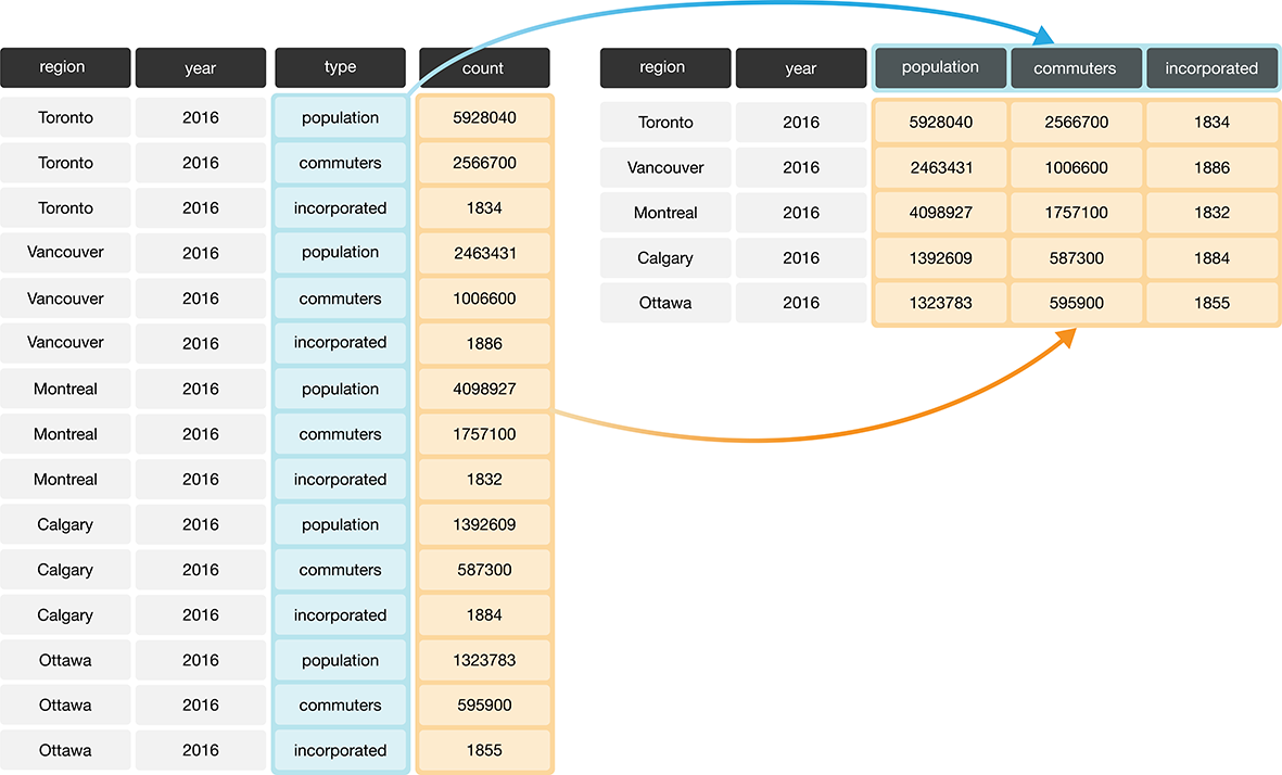
Figure 3.10: Going from long to wide data.
To tidy this type of data in R, we can use the pivot_wider function.
The pivot_wider function generally increases the number of columns (widens)
and decreases the number of rows in a data set.
To learn how to use pivot_wider,
we will work through an example
with the region_lang_top5_cities_long.csv data set.
This data set contains the number of Canadians reporting
the primary language at home and work for five
major cities (Toronto, Montréal, Vancouver, Calgary, and Edmonton).
## # A tibble: 2,140 × 5
##    region    category             language                     type         count
##    <chr>     <chr>                <chr>                        <chr>        <dbl>
##  1 Montréal  Aboriginal languages Aboriginal languages, n.o.s. most_at_home    15
##  2 Montréal  Aboriginal languages Aboriginal languages, n.o.s. most_at_work     0
##  3 Toronto   Aboriginal languages Aboriginal languages, n.o.s. most_at_home    50
##  4 Toronto   Aboriginal languages Aboriginal languages, n.o.s. most_at_work     0
##  5 Calgary   Aboriginal languages Aboriginal languages, n.o.s. most_at_home     5
##  6 Calgary   Aboriginal languages Aboriginal languages, n.o.s. most_at_work     0
##  7 Edmonton  Aboriginal languages Aboriginal languages, n.o.s. most_at_home    10
##  8 Edmonton  Aboriginal languages Aboriginal languages, n.o.s. most_at_work     0
##  9 Vancouver Aboriginal languages Aboriginal languages, n.o.s. most_at_home    15
## 10 Vancouver Aboriginal languages Aboriginal languages, n.o.s. most_at_work     0
## # ℹ 2,130 more rows
What makes the data set shown above untidy?
In this example, each observation is a language in a region.
However, each observation is split across multiple rows:
one where the count for most_at_home is recorded,
and the other where the count for most_at_work is recorded.
Suppose the goal with this data was to
visualize the relationship between the number of
Canadians reporting their primary language at home and work.
Doing that would be difficult with this data in its current form,
since these two variables are stored in the same column.
Figure 3.11 shows how this data
will be tidied using the pivot_wider function.
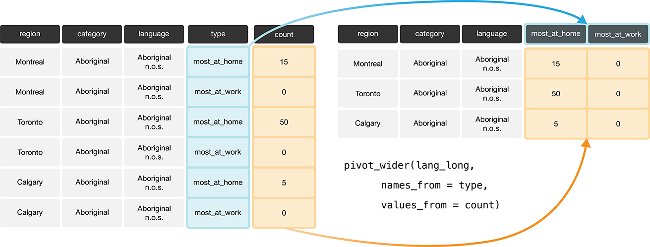
Figure 3.11: Going from long to wide with the pivot_wider function.
Figure 3.12 details the arguments that we need to specify
in the pivot_wider function.
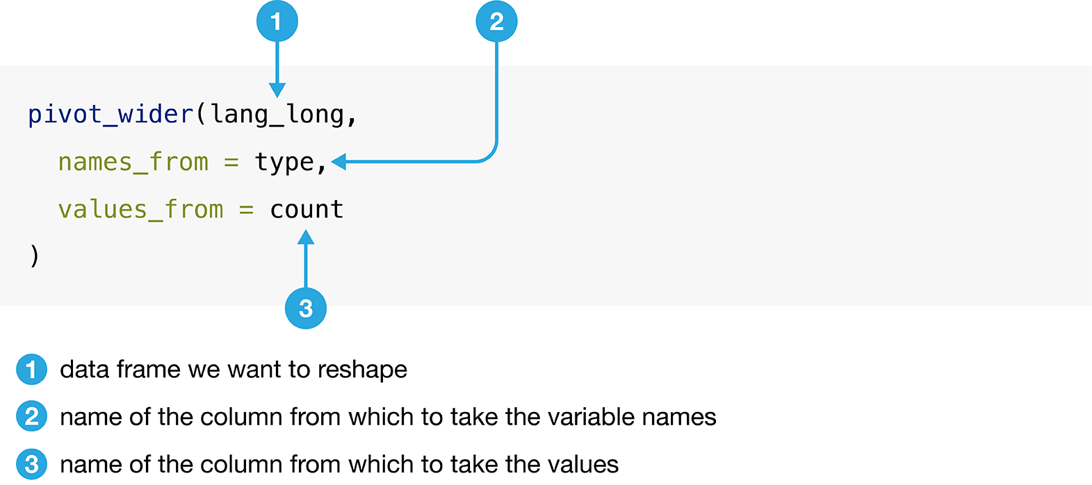
Figure 3.12: Syntax for the pivot_wider function.
We will apply the function as detailed in Figure 3.12.
## # A tibble: 1,070 × 5
##    region    category                         language most_at_home most_at_work
##    <chr>     <chr>                            <chr>           <dbl>        <dbl>
##  1 Montréal  Aboriginal languages             Aborigi…           15            0
##  2 Toronto   Aboriginal languages             Aborigi…           50            0
##  3 Calgary   Aboriginal languages             Aborigi…            5            0
##  4 Edmonton  Aboriginal languages             Aborigi…           10            0
##  5 Vancouver Aboriginal languages             Aborigi…           15            0
##  6 Montréal  Non-Official & Non-Aboriginal l… Afrikaa…           10            0
##  7 Toronto   Non-Official & Non-Aboriginal l… Afrikaa…          265            0
##  8 Calgary   Non-Official & Non-Aboriginal l… Afrikaa…          505           15
##  9 Edmonton  Non-Official & Non-Aboriginal l… Afrikaa…          300            0
## 10 Vancouver Non-Official & Non-Aboriginal l… Afrikaa…          520           10
## # ℹ 1,060 more rows
The data above is now tidy! We can go through the three criteria again to check that this data is a tidy data set.
- All the statistical variables are their own columns in the data frame (i.e.,
most_at_home, andmost_at_workhave been separated into their own columns in the data frame). - Each observation, (i.e., each language in a region) is in a single row.
- Each value is a single cell (i.e., its row, column position in the data frame is not shared with another value).
You might notice that we have the same number of columns in the tidy data set as
we did in the messy one. Therefore pivot_wider didn’t really “widen” the data,
as the name suggests. This is just because the original type column only had
two categories in it. If it had more than two, pivot_wider would have created
more columns, and we would see the data set “widen.”
3.4.3 Tidying up: using separate to deal with multiple delimiters
Data are also not considered tidy when multiple values are stored in the same
cell. The data set we show below is even messier than the ones we dealt with
above: the Toronto, Montréal, Vancouver, Calgary, and Edmonton columns
contain the number of Canadians reporting their primary language at home and
work in one column separated by the delimiter (/). The column names are the
values of a variable, and each value does not have its own cell! To turn this
messy data into tidy data, we’ll have to fix these issues.
## # A tibble: 214 × 7
## category language Toronto Montréal Vancouver Calgary Edmonton
## <chr> <chr> <chr> <chr> <chr> <chr> <chr>
## 1 Aboriginal languages Aborigi… 50/0 15/0 15/0 5/0 10/0
## 2 Non-Official & Non-Abor… Afrikaa… 265/0 10/0 520/10 505/15 300/0
## 3 Non-Official & Non-Abor… Afro-As… 185/10 65/0 10/0 15/0 20/0
## 4 Non-Official & Non-Abor… Akan (T… 4045/20 440/0 125/10 330/0 445/0
## 5 Non-Official & Non-Abor… Albanian 6380/2… 1445/20 530/10 620/25 370/10
## 6 Aboriginal languages Algonqu… 5/0 0/0 0/0 0/0 0/0
## 7 Aboriginal languages Algonqu… 0/0 10/0 0/0 0/0 0/0
## 8 Non-Official & Non-Abor… America… 720/245 70/0 300/140 85/25 190/85
## 9 Non-Official & Non-Abor… Amharic 3820/55 315/0 540/10 2730/50 1695/35
## 10 Non-Official & Non-Abor… Arabic 45025/… 72980/1… 8680/275 11010/… 10590/3…
## # ℹ 204 more rowsFirst we’ll use pivot_longer to create two columns, region and value,
similar to what we did previously.
The new region columns will contain the region names,
and the new column value will be a temporary holding place for the
data that we need to further separate, i.e., the
number of Canadians reporting their primary language at home and work.
lang_messy_longer <- pivot_longer(lang_messy,
cols = Toronto:Edmonton,
names_to = "region",
values_to = "value"
)
lang_messy_longer## # A tibble: 1,070 × 4
## category language region value
## <chr> <chr> <chr> <chr>
## 1 Aboriginal languages Aboriginal languages, n… Toron… 50/0
## 2 Aboriginal languages Aboriginal languages, n… Montr… 15/0
## 3 Aboriginal languages Aboriginal languages, n… Vanco… 15/0
## 4 Aboriginal languages Aboriginal languages, n… Calga… 5/0
## 5 Aboriginal languages Aboriginal languages, n… Edmon… 10/0
## 6 Non-Official & Non-Aboriginal languages Afrikaans Toron… 265/0
## 7 Non-Official & Non-Aboriginal languages Afrikaans Montr… 10/0
## 8 Non-Official & Non-Aboriginal languages Afrikaans Vanco… 520/…
## 9 Non-Official & Non-Aboriginal languages Afrikaans Calga… 505/…
## 10 Non-Official & Non-Aboriginal languages Afrikaans Edmon… 300/0
## # ℹ 1,060 more rowsNext we’ll use separate to split the value column into two columns.
One column will contain only the counts of Canadians
that speak each language most at home,
and the other will contain the counts of Canadians
that speak each language most at work for each region.
Figure 3.13
outlines what we need to specify to use separate.
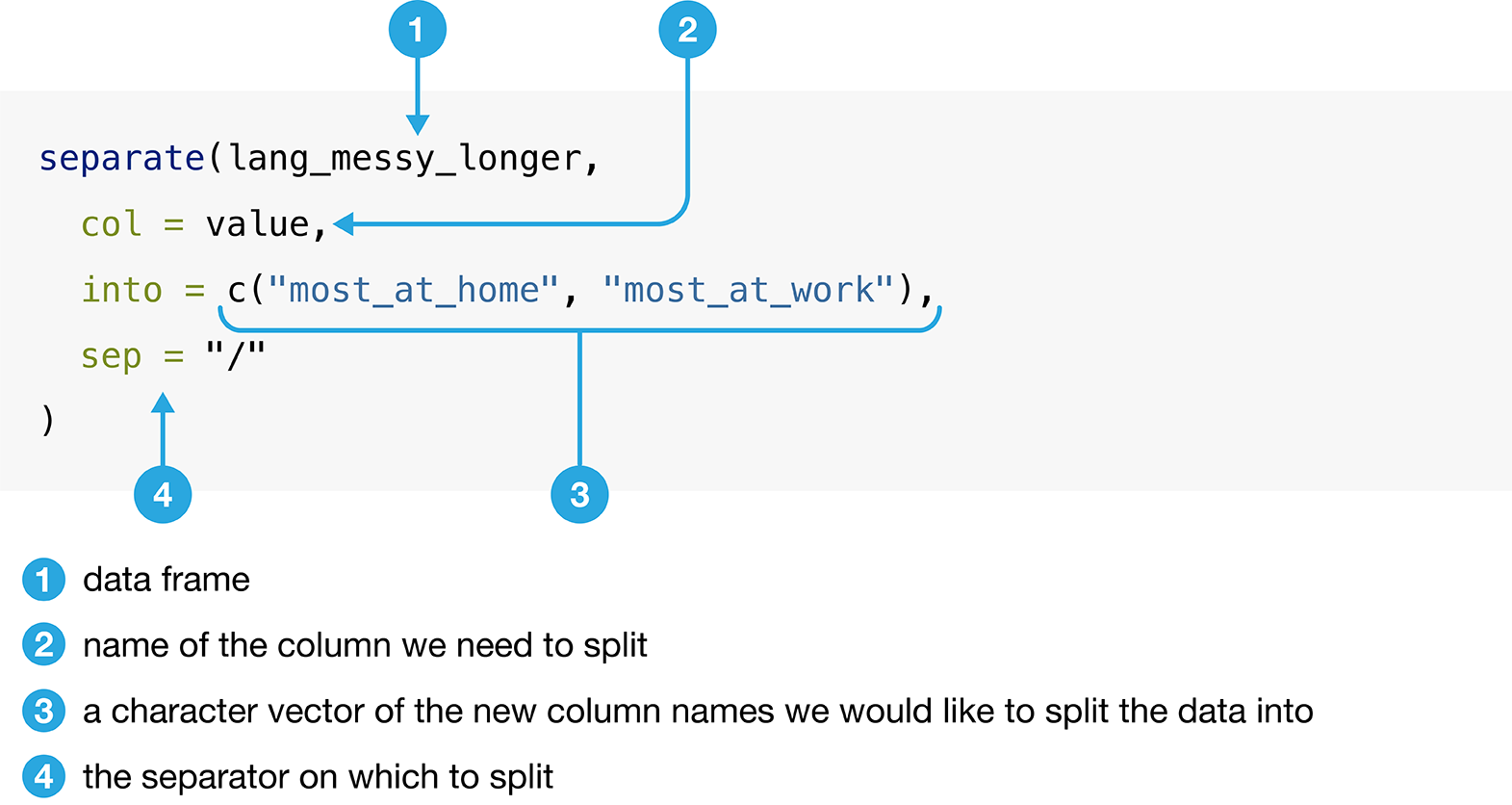
Figure 3.13: Syntax for the separate function.
tidy_lang <- separate(lang_messy_longer,
col = value,
into = c("most_at_home", "most_at_work"),
sep = "/"
)
tidy_lang## # A tibble: 1,070 × 5
## category language region most_at_home most_at_work
## <chr> <chr> <chr> <chr> <chr>
## 1 Aboriginal languages Aborigi… Toron… 50 0
## 2 Aboriginal languages Aborigi… Montr… 15 0
## 3 Aboriginal languages Aborigi… Vanco… 15 0
## 4 Aboriginal languages Aborigi… Calga… 5 0
## 5 Aboriginal languages Aborigi… Edmon… 10 0
## 6 Non-Official & Non-Aboriginal lang… Afrikaa… Toron… 265 0
## 7 Non-Official & Non-Aboriginal lang… Afrikaa… Montr… 10 0
## 8 Non-Official & Non-Aboriginal lang… Afrikaa… Vanco… 520 10
## 9 Non-Official & Non-Aboriginal lang… Afrikaa… Calga… 505 15
## 10 Non-Official & Non-Aboriginal lang… Afrikaa… Edmon… 300 0
## # ℹ 1,060 more rowsIs this data set now tidy? If we recall the three criteria for tidy data:
- each row is a single observation,
- each column is a single variable, and
- each value is a single cell.
We can see that this data now satisfies all three criteria, making it easier to
analyze. But we aren’t done yet! Notice in the table above that the word
<chr> appears beneath each of the column names. The word under the column name
indicates the data type of each column. Here all of the variables are
“character” data types. Recall, character data types are letter(s) or digits(s)
surrounded by quotes. In the previous example in Section 3.4.2, the
most_at_home and most_at_work variables were <dbl> (double)—you can
verify this by looking at the tables in the previous sections—which is a type
of numeric data. This change is due to the delimiter (/) when we read in this
messy data set. R read these columns in as character types, and by default,
separate will return columns as character data types.
It makes sense for region, category, and language to be stored as a
character (or perhaps factor) type. However, suppose we want to apply any functions that treat the
most_at_home and most_at_work columns as a number (e.g., finding rows
above a numeric threshold of a column).
In that case,
it won’t be possible to do if the variable is stored as a character.
Fortunately, the separate function provides a natural way to fix problems
like this: we can set convert = TRUE to convert the most_at_home
and most_at_work columns to the correct data type.
tidy_lang <- separate(lang_messy_longer,
col = value,
into = c("most_at_home", "most_at_work"),
sep = "/",
convert = TRUE
)
tidy_lang## # A tibble: 1,070 × 5
## category language region most_at_home most_at_work
## <chr> <chr> <chr> <int> <int>
## 1 Aboriginal languages Aborigi… Toron… 50 0
## 2 Aboriginal languages Aborigi… Montr… 15 0
## 3 Aboriginal languages Aborigi… Vanco… 15 0
## 4 Aboriginal languages Aborigi… Calga… 5 0
## 5 Aboriginal languages Aborigi… Edmon… 10 0
## 6 Non-Official & Non-Aboriginal lang… Afrikaa… Toron… 265 0
## 7 Non-Official & Non-Aboriginal lang… Afrikaa… Montr… 10 0
## 8 Non-Official & Non-Aboriginal lang… Afrikaa… Vanco… 520 10
## 9 Non-Official & Non-Aboriginal lang… Afrikaa… Calga… 505 15
## 10 Non-Official & Non-Aboriginal lang… Afrikaa… Edmon… 300 0
## # ℹ 1,060 more rowsNow we see <int> appears under the most_at_home and most_at_work columns,
indicating they are integer data types (i.e., numbers)!
3.5 Using select to extract a range of columns
Now that the tidy_lang data is indeed tidy, we can start manipulating it
using the powerful suite of functions from the tidyverse.
For the first example, recall the select function from Chapter 1,
which lets us create a subset of columns from a data frame.
Suppose we wanted to select only the columns language, region,
most_at_home and most_at_work from the tidy_lang data set. Using what we
learned in Chapter 1, we would pass the tidy_lang data frame as
well as all of these column names into the select function:
selected_columns <- select(tidy_lang,
language,
region,
most_at_home,
most_at_work)
selected_columns## # A tibble: 1,070 × 4
## language region most_at_home most_at_work
## <chr> <chr> <int> <int>
## 1 Aboriginal languages, n.o.s. Toronto 50 0
## 2 Aboriginal languages, n.o.s. Montréal 15 0
## 3 Aboriginal languages, n.o.s. Vancouver 15 0
## 4 Aboriginal languages, n.o.s. Calgary 5 0
## 5 Aboriginal languages, n.o.s. Edmonton 10 0
## 6 Afrikaans Toronto 265 0
## 7 Afrikaans Montréal 10 0
## 8 Afrikaans Vancouver 520 10
## 9 Afrikaans Calgary 505 15
## 10 Afrikaans Edmonton 300 0
## # ℹ 1,060 more rowsHere we wrote out the names of each of the columns. However, this method is
time-consuming, especially if you have a lot of columns! Another approach is to
use a “select helper”. Select helpers are operators that make it easier for
us to select columns. For instance, we can use a select helper to choose a
range of columns rather than typing each column name out. To do this, we use the
colon (:) operator to denote the range. For example, to get all the columns in
the tidy_lang data frame from language to most_at_work we pass
language:most_at_work as the second argument to the select function.
## # A tibble: 1,070 × 4
## language region most_at_home most_at_work
## <chr> <chr> <int> <int>
## 1 Aboriginal languages, n.o.s. Toronto 50 0
## 2 Aboriginal languages, n.o.s. Montréal 15 0
## 3 Aboriginal languages, n.o.s. Vancouver 15 0
## 4 Aboriginal languages, n.o.s. Calgary 5 0
## 5 Aboriginal languages, n.o.s. Edmonton 10 0
## 6 Afrikaans Toronto 265 0
## 7 Afrikaans Montréal 10 0
## 8 Afrikaans Vancouver 520 10
## 9 Afrikaans Calgary 505 15
## 10 Afrikaans Edmonton 300 0
## # ℹ 1,060 more rowsNotice that we get the same output as we did above, but with less (and clearer!) code. This type of operator is especially handy for large data sets.
Suppose instead we wanted to extract columns that followed a particular pattern
rather than just selecting a range. For example, let’s say we wanted only to select the
columns most_at_home and most_at_work. There are other helpers that allow
us to select variables based on their names. In particular, we can use the select helper
starts_with to choose only the columns that start with the word “most”:
## # A tibble: 1,070 × 2
## most_at_home most_at_work
## <int> <int>
## 1 50 0
## 2 15 0
## 3 15 0
## 4 5 0
## 5 10 0
## 6 265 0
## 7 10 0
## 8 520 10
## 9 505 15
## 10 300 0
## # ℹ 1,060 more rowsWe could also have chosen the columns containing an underscore _ by adding
contains("_") as the second argument in the select function, since we notice
the columns we want contain underscores and the others don’t.
## # A tibble: 1,070 × 2
## most_at_home most_at_work
## <int> <int>
## 1 50 0
## 2 15 0
## 3 15 0
## 4 5 0
## 5 10 0
## 6 265 0
## 7 10 0
## 8 520 10
## 9 505 15
## 10 300 0
## # ℹ 1,060 more rowsThere are many different select helpers that select
variables based on certain criteria.
The additional resources section at the end of this chapter
provides a comprehensive resource on select helpers.
3.6 Using filter to extract rows
Next, we revisit the filter function from Chapter 1,
which lets us create a subset of rows from a data frame.
Recall the two main arguments to the filter function:
the first is the name of the data frame object, and
the second is a logical statement to use when filtering the rows.
filter works by returning the rows where the logical statement evaluates to TRUE.
This section will highlight more advanced usage of the filter function.
In particular, this section provides an in-depth treatment of the variety of logical statements
one can use in the filter function to select subsets of rows.
3.6.1 Extracting rows that have a certain value with ==
Suppose we are only interested in the subset of rows in tidy_lang corresponding to the
official languages of Canada (English and French).
We can filter for these rows by using the equivalency operator (==)
to compare the values of the category column
with the value "Official languages".
With these arguments, filter returns a data frame with all the columns
of the input data frame
but only the rows we asked for in the logical statement, i.e.,
those where the category column holds the value "Official languages".
We name this data frame official_langs.
## # A tibble: 10 × 5
## category language region most_at_home most_at_work
## <chr> <chr> <chr> <int> <int>
## 1 Official languages English Toronto 3836770 3218725
## 2 Official languages English Montréal 620510 412120
## 3 Official languages English Vancouver 1622735 1330555
## 4 Official languages English Calgary 1065070 844740
## 5 Official languages English Edmonton 1050410 792700
## 6 Official languages French Toronto 29800 11940
## 7 Official languages French Montréal 2669195 1607550
## 8 Official languages French Vancouver 8630 3245
## 9 Official languages French Calgary 8630 2140
## 10 Official languages French Edmonton 10950 25203.6.2 Extracting rows that do not have a certain value with !=
What if we want all the other language categories in the data set except for
those in the "Official languages" category? We can accomplish this with the !=
operator, which means “not equal to”. So if we want to find all the rows
where the category does not equal "Official languages" we write the code
below.
## # A tibble: 1,060 × 5
## category language region most_at_home most_at_work
## <chr> <chr> <chr> <int> <int>
## 1 Aboriginal languages Aborigi… Toron… 50 0
## 2 Aboriginal languages Aborigi… Montr… 15 0
## 3 Aboriginal languages Aborigi… Vanco… 15 0
## 4 Aboriginal languages Aborigi… Calga… 5 0
## 5 Aboriginal languages Aborigi… Edmon… 10 0
## 6 Non-Official & Non-Aboriginal lang… Afrikaa… Toron… 265 0
## 7 Non-Official & Non-Aboriginal lang… Afrikaa… Montr… 10 0
## 8 Non-Official & Non-Aboriginal lang… Afrikaa… Vanco… 520 10
## 9 Non-Official & Non-Aboriginal lang… Afrikaa… Calga… 505 15
## 10 Non-Official & Non-Aboriginal lang… Afrikaa… Edmon… 300 0
## # ℹ 1,050 more rows3.6.3 Extracting rows satisfying multiple conditions using , or &
Suppose now we want to look at only the rows
for the French language in Montréal.
To do this, we need to filter the data set
to find rows that satisfy multiple conditions simultaneously.
We can do this with the comma symbol (,), which in the case of filter
is interpreted by R as “and”.
We write the code as shown below to filter the official_langs data frame
to subset the rows where region == "Montréal"
and the language == "French".
## # A tibble: 1 × 5
## category language region most_at_home most_at_work
## <chr> <chr> <chr> <int> <int>
## 1 Official languages French Montréal 2669195 1607550We can also use the ampersand (&) logical operator, which gives
us cases where both one condition and another condition
are satisfied. You can use either comma (,) or ampersand (&) in the filter
function interchangeably.
## # A tibble: 1 × 5
## category language region most_at_home most_at_work
## <chr> <chr> <chr> <int> <int>
## 1 Official languages French Montréal 2669195 16075503.6.4 Extracting rows satisfying at least one condition using |
Suppose we were interested in only those rows corresponding to cities in Alberta
in the official_langs data set (Edmonton and Calgary).
We can’t use , as we did above because region
cannot be both Edmonton and Calgary simultaneously.
Instead, we can use the vertical pipe (|) logical operator,
which gives us the cases where one condition or
another condition or both are satisfied.
In the code below, we ask R to return the rows
where the region columns are equal to “Calgary” or “Edmonton”.
## # A tibble: 4 × 5
## category language region most_at_home most_at_work
## <chr> <chr> <chr> <int> <int>
## 1 Official languages English Calgary 1065070 844740
## 2 Official languages English Edmonton 1050410 792700
## 3 Official languages French Calgary 8630 2140
## 4 Official languages French Edmonton 10950 25203.6.5 Extracting rows with values in a vector using %in%
Next, suppose we want to see the populations of our five cities.
Let’s read in the region_data.csv file
that comes from the 2016 Canadian census,
as it contains statistics for number of households, land area, population
and number of dwellings for different regions.
## # A tibble: 35 × 5
## region households area population dwellings
## <chr> <dbl> <dbl> <dbl> <dbl>
## 1 Belleville 43002 1355. 103472 45050
## 2 Lethbridge 45696 3047. 117394 48317
## 3 Thunder Bay 52545 2618. 121621 57146
## 4 Peterborough 50533 1637. 121721 55662
## 5 Saint John 52872 3793. 126202 58398
## 6 Brantford 52530 1086. 134203 54419
## 7 Moncton 61769 2625. 144810 66699
## 8 Guelph 59280 604. 151984 63324
## 9 Trois-Rivières 72502 1053. 156042 77734
## 10 Saguenay 72479 3079. 160980 77968
## # ℹ 25 more rowsTo get the population of the five cities
we can filter the data set using the %in% operator.
The %in% operator is used to see if an element belongs to a vector.
Here we are filtering for rows where the value in the region column
matches any of the five cities we are intersted in: Toronto, Montréal,
Vancouver, Calgary, and Edmonton.
city_names <- c("Toronto", "Montréal", "Vancouver", "Calgary", "Edmonton")
five_cities <- filter(region_data,
region %in% city_names)
five_cities## # A tibble: 5 × 5
## region households area population dwellings
## <chr> <dbl> <dbl> <dbl> <dbl>
## 1 Edmonton 502143 9858. 1321426 537634
## 2 Calgary 519693 5242. 1392609 544870
## 3 Vancouver 960894 3040. 2463431 1027613
## 4 Montréal 1727310 4638. 4098927 1823281
## 5 Toronto 2135909 6270. 5928040 2235145Note: What’s the difference between
==and%in%? Suppose we have two vectors,vectorAandvectorB. If you typevectorA == vectorBinto R it will compare the vectors element by element. R checks if the first element ofvectorAequals the first element ofvectorB, the second element ofvectorAequals the second element ofvectorB, and so on. On the other hand,vectorA %in% vectorBcompares the first element ofvectorAto all the elements invectorB. Then the second element ofvectorAis compared to all the elements invectorB, and so on. Notice the difference between==and%in%in the example below.## [1] FALSE FALSE## [1] TRUE TRUE
3.6.6 Extracting rows above or below a threshold using > and <
We saw in Section 3.6.3 that
2,669,195 people reported
speaking French in Montréal as their primary language at home.
If we are interested in finding the official languages in regions
with higher numbers of people who speak it as their primary language at home
compared to French in Montréal, then we can use filter to obtain rows
where the value of most_at_home is greater than
2,669,195.
We use the > symbol to look for values above a threshold, and the < symbol
to look for values below a threshold. The >= and <= symbols similarly look
for equal to or above a threshold and equal to or below a
threshold.
## # A tibble: 1 × 5
## category language region most_at_home most_at_work
## <chr> <chr> <chr> <int> <int>
## 1 Official languages English Toronto 3836770 3218725filter returns a data frame with only one row, indicating that when
considering the official languages,
only English in Toronto is reported by more people
as their primary language at home
than French in Montréal according to the 2016 Canadian census.
3.7 Using mutate to modify or add columns
3.7.1 Using mutate to modify columns
In Section 3.4.3,
when we first read in the "region_lang_top5_cities_messy.csv" data,
all of the variables were “character” data types.
During the tidying process,
we used the convert argument from the separate function
to convert the most_at_home and most_at_work columns
to the desired integer (i.e., numeric class) data types.
But suppose we didn’t use the convert argument,
and needed to modify the column type some other way.
Below we create such a situation
so that we can demonstrate how to use mutate
to change the column types of a data frame.
mutate is a useful function to modify or create new data frame columns.
lang_messy <- read_csv("data/region_lang_top5_cities_messy.csv")
lang_messy_longer <- pivot_longer(lang_messy,
cols = Toronto:Edmonton,
names_to = "region",
values_to = "value")
tidy_lang_chr <- separate(lang_messy_longer, col = value,
into = c("most_at_home", "most_at_work"),
sep = "/")
official_langs_chr <- filter(tidy_lang_chr, category == "Official languages")
official_langs_chr## # A tibble: 10 × 5
## category language region most_at_home most_at_work
## <chr> <chr> <chr> <chr> <chr>
## 1 Official languages English Toronto 3836770 3218725
## 2 Official languages English Montréal 620510 412120
## 3 Official languages English Vancouver 1622735 1330555
## 4 Official languages English Calgary 1065070 844740
## 5 Official languages English Edmonton 1050410 792700
## 6 Official languages French Toronto 29800 11940
## 7 Official languages French Montréal 2669195 1607550
## 8 Official languages French Vancouver 8630 3245
## 9 Official languages French Calgary 8630 2140
## 10 Official languages French Edmonton 10950 2520To use mutate, again we first specify the data set in the first argument,
and in the following arguments,
we specify the name of the column we want to modify or create
(here most_at_home and most_at_work), an = sign,
and then the function we want to apply (here as.numeric).
In the function we want to apply,
we refer directly to the column name upon which we want it to act
(here most_at_home and most_at_work).
In our example, we are naming the columns the same
names as columns that already exist in the data frame
(“most_at_home”, “most_at_work”)
and this will cause mutate to overwrite those columns
(also referred to as modifying those columns in-place).
If we were to give the columns a new name,
then mutate would create new columns with the names we specified.
mutate’s general syntax is detailed in Figure 3.14.
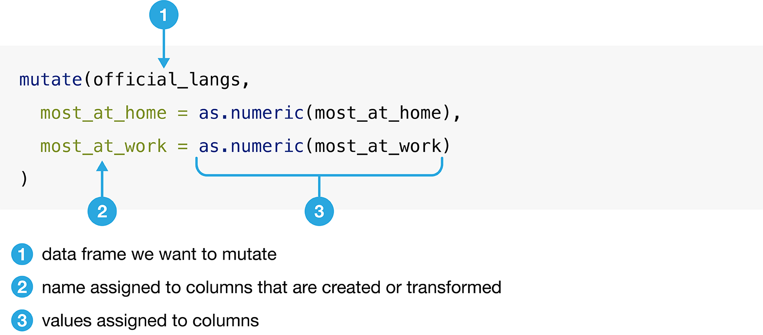
Figure 3.14: Syntax for the mutate function.
Below we use mutate to convert the columns most_at_home and most_at_work
to numeric data types in the official_langs data set as described in Figure
3.14:
official_langs_numeric <- mutate(official_langs_chr,
most_at_home = as.numeric(most_at_home),
most_at_work = as.numeric(most_at_work)
)
official_langs_numeric## # A tibble: 10 × 5
## category language region most_at_home most_at_work
## <chr> <chr> <chr> <dbl> <dbl>
## 1 Official languages English Toronto 3836770 3218725
## 2 Official languages English Montréal 620510 412120
## 3 Official languages English Vancouver 1622735 1330555
## 4 Official languages English Calgary 1065070 844740
## 5 Official languages English Edmonton 1050410 792700
## 6 Official languages French Toronto 29800 11940
## 7 Official languages French Montréal 2669195 1607550
## 8 Official languages French Vancouver 8630 3245
## 9 Official languages French Calgary 8630 2140
## 10 Official languages French Edmonton 10950 2520Now we see <dbl> appears under the most_at_home and most_at_work columns,
indicating they are double data types (which is a numeric data type)!
3.7.2 Using mutate to create new columns
We can see in the table that 3,836,770 people reported speaking English in Toronto as their primary language at home, according to the 2016 Canadian census. What does this number mean to us? To understand this number, we need context. In particular, how many people were in Toronto when this data was collected? From the 2016 Canadian census profile, the population of Toronto was reported to be 5,928,040 people. The number of people who report that English is their primary language at home is much more meaningful when we report it in this context. We can even go a step further and transform this count to a relative frequency or proportion. We can do this by dividing the number of people reporting a given language as their primary language at home by the number of people who live in Toronto. For example, the proportion of people who reported that their primary language at home was English in the 2016 Canadian census was 0.65 in Toronto.
Let’s use mutate to create a new column in our data frame
that holds the proportion of people who speak English
for our five cities of focus in this chapter.
To accomplish this, we will need to do two tasks
beforehand:
- Create a vector containing the population values for the cities.
- Filter the
official_langsdata frame so that we only keep the rows where the language is English.
To create a vector containing the population values for the five cities
(Toronto, Montréal, Vancouver, Calgary, Edmonton),
we will use the c function (recall that c stands for “concatenate”):
## [1] 5928040 4098927 2463431 1392609 1321426And next, we will filter the official_langs data frame
so that we only keep the rows where the language is English.
We will name the new data frame we get from this english_langs:
## # A tibble: 5 × 5
## category language region most_at_home most_at_work
## <chr> <chr> <chr> <int> <int>
## 1 Official languages English Toronto 3836770 3218725
## 2 Official languages English Montréal 620510 412120
## 3 Official languages English Vancouver 1622735 1330555
## 4 Official languages English Calgary 1065070 844740
## 5 Official languages English Edmonton 1050410 792700Finally, we can use mutate to create a new column,
named most_at_home_proportion, that will have value that corresponds to
the proportion of people reporting English as their primary
language at home.
We will compute this by dividing the column by our vector of city populations.
english_langs <- mutate(english_langs,
most_at_home_proportion = most_at_home / city_pops)
english_langs## # A tibble: 5 × 6
## category language region most_at_home most_at_work most_at_home_proport…¹
## <chr> <chr> <chr> <int> <int> <dbl>
## 1 Official lan… English Toron… 3836770 3218725 0.647
## 2 Official lan… English Montr… 620510 412120 0.151
## 3 Official lan… English Vanco… 1622735 1330555 0.659
## 4 Official lan… English Calga… 1065070 844740 0.765
## 5 Official lan… English Edmon… 1050410 792700 0.795
## # ℹ abbreviated name: ¹most_at_home_proportionIn the computation above, we had to ensure that we ordered the city_pops vector in the
same order as the cities were listed in the english_langs data frame.
This is because R will perform the division computation we did by dividing
each element of the most_at_home column by each element of the
city_pops vector, matching them up by position.
Failing to do this would have resulted in the incorrect math being performed.
Note: In more advanced data wrangling, one might solve this problem in a less error-prone way though using a technique called “joins.” We link to resources that discuss this in the additional resources at the end of this chapter.
3.8 Combining functions using the pipe operator, |>
In R, we often have to call multiple functions in a sequence to process a data
frame. The basic ways of doing this can become quickly unreadable if there are
many steps. For example, suppose we need to perform three operations on a data
frame called data:
- add a new column
new_colthat is double anotherold_col, - filter for rows where another column,
other_col, is more than 5, and - select only the new column
new_colfor those rows.
One way of performing these three steps is to just write multiple lines of code, storing temporary objects as you go:
output_1 <- mutate(data, new_col = old_col * 2)
output_2 <- filter(output_1, other_col > 5)
output <- select(output_2, new_col)This is difficult to understand for multiple reasons. The reader may be tricked
into thinking the named output_1 and output_2 objects are important for some
reason, while they are just temporary intermediate computations. Further, the
reader has to look through and find where output_1 and output_2 are used in
each subsequent line.
Another option for doing this would be to compose the functions:
Code like this can also be difficult to understand. Functions compose (reading
from left to right) in the opposite order in which they are computed by R
(above, mutate happens first, then filter, then select). It is also just a
really long line of code to read in one go.
The pipe operator (|>) solves this problem, resulting in cleaner and
easier-to-follow code. |> is built into R so you don’t need to load any
packages to use it.
You can think of the pipe as a physical pipe. It takes the output from the
function on the left-hand side of the pipe, and passes it as the first argument
to the function on the right-hand side of the pipe.
The code below accomplishes the same thing as the previous
two code blocks:
Note: You might also have noticed that we split the function calls across lines after the pipe, similar to when we did this earlier in the chapter for long function calls. Again, this is allowed and recommended, especially when the piped function calls create a long line of code. Doing this makes your code more readable. When you do this, it is important to end each line with the pipe operator
|>to tell R that your code is continuing onto the next line.
Note: In this textbook, we will be using the base R pipe operator syntax,
|>. This base R|>pipe operator was inspired by a previous version of the pipe operator,%>%. The%>%pipe operator is not built into R and is from themagrittrR package. Thetidyversemetapackage imports the%>%pipe operator viadplyr(which in turn imports themagrittrR package). There are some other differences between%>%and|>related to more advanced R uses, such as sharing and distributing code as R packages, however, these are beyond the scope of this textbook. We have this note in the book to make the reader aware that%>%exists as it is still commonly used in data analysis code and in many data science books and other resources. In most cases these two pipes are interchangeable and either can be used.
3.8.1 Using |> to combine filter and select
Let’s work with the tidy tidy_lang data set from Section 3.4.3,
which contains the number of Canadians reporting their primary language at home
and work for five major cities
(Toronto, Montréal, Vancouver, Calgary, and Edmonton):
## # A tibble: 1,070 × 5
##    category                            language region most_at_home most_at_work
##    <chr>                               <chr>    <chr>         <int>        <int>
##  1 Aboriginal languages                Aborigi… Toron…           50            0
##  2 Aboriginal languages                Aborigi… Montr…           15            0
##  3 Aboriginal languages                Aborigi… Vanco…           15            0
##  4 Aboriginal languages                Aborigi… Calga…            5            0
##  5 Aboriginal languages                Aborigi… Edmon…           10            0
##  6 Non-Official & Non-Aboriginal lang… Afrikaa… Toron…          265            0
##  7 Non-Official & Non-Aboriginal lang… Afrikaa… Montr…           10            0
##  8 Non-Official & Non-Aboriginal lang… Afrikaa… Vanco…          520           10
##  9 Non-Official & Non-Aboriginal lang… Afrikaa… Calga…          505           15
## 10 Non-Official & Non-Aboriginal lang… Afrikaa… Edmon…          300            0
## # ℹ 1,060 more rowsSuppose we want to create a subset of the data with only the languages and
counts of each language spoken most at home for the city of Vancouver. To do
this, we can use the functions filter and select. First, we use filter to
create a data frame called van_data that contains only values for Vancouver.
## # A tibble: 214 × 5
##    category                            language region most_at_home most_at_work
##    <chr>                               <chr>    <chr>         <int>        <int>
##  1 Aboriginal languages                Aborigi… Vanco…           15            0
##  2 Non-Official & Non-Aboriginal lang… Afrikaa… Vanco…          520           10
##  3 Non-Official & Non-Aboriginal lang… Afro-As… Vanco…           10            0
##  4 Non-Official & Non-Aboriginal lang… Akan (T… Vanco…          125           10
##  5 Non-Official & Non-Aboriginal lang… Albanian Vanco…          530           10
##  6 Aboriginal languages                Algonqu… Vanco…            0            0
##  7 Aboriginal languages                Algonqu… Vanco…            0            0
##  8 Non-Official & Non-Aboriginal lang… America… Vanco…          300          140
##  9 Non-Official & Non-Aboriginal lang… Amharic  Vanco…          540           10
## 10 Non-Official & Non-Aboriginal lang… Arabic   Vanco…         8680          275
## # ℹ 204 more rows
We then use select on this data frame to keep only the variables we want:
## # A tibble: 214 × 2
##    language                       most_at_home
##    <chr>                                 <int>
##  1 Aboriginal languages, n.o.s.             15
##  2 Afrikaans                               520
##  3 Afro-Asiatic languages, n.i.e.           10
##  4 Akan (Twi)                              125
##  5 Albanian                                530
##  6 Algonquian languages, n.i.e.              0
##  7 Algonquin                                 0
##  8 American Sign Language                  300
##  9 Amharic                                 540
## 10 Arabic                                 8680
## # ℹ 204 more rows
Although this is valid code, there is a more readable approach we could take by
using the pipe, |>. With the pipe, we do not need to create an intermediate
object to store the output from filter. Instead, we can directly send the
output of filter to the input of select:
van_data_selected <- filter(tidy_lang, region == "Vancouver") |>
        select(language, most_at_home)

van_data_selected
## # A tibble: 214 × 2
## language most_at_home
## <chr> <int>
## 1 Aboriginal languages, n.o.s. 15
## 2 Afrikaans 520
## 3 Afro-Asiatic languages, n.i.e. 10
## 4 Akan (Twi) 125
## 5 Albanian 530
## 6 Algonquian languages, n.i.e. 0
## 7 Algonquin 0
## 8 American Sign Language 300
## 9 Amharic 540
## 10 Arabic 8680
## # ℹ 204 more rowsBut wait…Why do the select function calls
look different in these two examples?
Remember: when you use the pipe,
the output of the first function is automatically provided
as the first argument for the function that comes after it.
Therefore you do not specify the first argument in that function call.
In the code above,
The pipe passes the left-hand side (the output of filter) to the first argument of the function on the right (select),
so in the select function you only see the second argument (and beyond).
As you can see, both of these approaches—with and without pipes—give us the same output, but the second
approach is clearer and more readable.
3.8.2 Using |> with more than two functions
The pipe operator (|>) can be used with any function in R. Additionally, we can pipe together more than two functions. For example, we can pipe together three functions to:
filterrows to include only those where the counts of the language most spoken at home are greater than 10,000,selectonly the columns corresponding toregion,languageandmost_at_home, andarrangethe data frame rows in order by counts of the language most spoken at home from smallest to largest.
As we saw in Chapter 1,
we can use the tidyverse arrange function
to order the rows in the data frame by the values of one or more columns.
Here we pass the column name most_at_home to arrange the data frame rows by the values in that column, in ascending order.
large_region_lang <- filter(tidy_lang, most_at_home > 10000) |>
  select(region, language, most_at_home) |>
  arrange(most_at_home)

large_region_lang
## # A tibble: 67 × 3
## region language most_at_home
## <chr> <chr> <int>
## 1 Edmonton Arabic 10590
## 2 Montréal Tamil 10670
## 3 Vancouver Russian 10795
## 4 Edmonton Spanish 10880
## 5 Edmonton French 10950
## 6 Calgary Arabic 11010
## 7 Calgary Urdu 11060
## 8 Vancouver Hindi 11235
## 9 Montréal Armenian 11835
## 10 Toronto Romanian 12200
## # ℹ 57 more rowsYou will notice above that we passed tidy_lang as the first argument of the filter function.
We can also pipe the data frame into the same sequence of functions rather than
using it as the first argument of the first function. These two choices are equivalent,
and we get the same result.
large_region_lang <- tidy_lang |>
  filter(most_at_home > 10000) |>
  select(region, language, most_at_home) |>
  arrange(most_at_home)

large_region_lang
## # A tibble: 67 × 3
## region language most_at_home
## <chr> <chr> <int>
## 1 Edmonton Arabic 10590
## 2 Montréal Tamil 10670
## 3 Vancouver Russian 10795
## 4 Edmonton Spanish 10880
## 5 Edmonton French 10950
## 6 Calgary Arabic 11010
## 7 Calgary Urdu 11060
## 8 Vancouver Hindi 11235
## 9 Montréal Armenian 11835
## 10 Toronto Romanian 12200
## # ℹ 57 more rowsNow that we’ve shown you the pipe operator as an alternative to storing temporary objects and composing code, does this mean you should never store temporary objects or compose code? Not necessarily! There are times when you will still want to do these things. For example, you might store a temporary object before feeding it into a plot function so you can iteratively change the plot without having to redo all of your data transformations. Additionally, piping many functions can be overwhelming and difficult to debug; you may want to store a temporary object midway through to inspect your result before moving on with further steps.
3.9 Aggregating data with summarize and map
3.9.1 Calculating summary statistics on whole columns
As a part of many data analyses, we need to calculate a summary value for the data (a summary statistic). Examples of summary statistics we might want to calculate are the number of observations, the average/mean value for a column, the minimum value, etc. Oftentimes, this summary statistic is calculated from the values in a data frame column, or columns, as shown in Figure 3.15.
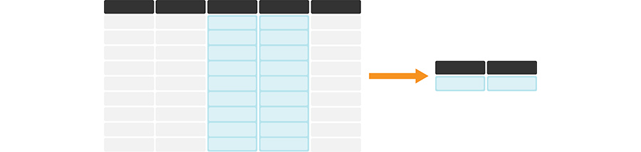
Figure 3.15: summarize is useful for calculating summary statistics on one or more column(s). In its simplest use case, it creates a new data frame with a single row containing the summary statistic(s) for each column being summarized. The darker, top row of each table represents the column headers.
A useful dplyr function for calculating summary statistics is summarize,
where the first argument is the data frame and subsequent arguments
are the summaries we want to perform.
Here we show how to use the summarize function to calculate the minimum
and maximum number of Canadians
reporting a particular language as their primary language at home.
First a reminder of what region_lang looks like:
## # A tibble: 7,490 × 7
##    region   category language mother_tongue most_at_home most_at_work lang_known
##    <chr>    <chr>    <chr>            <dbl>        <dbl>        <dbl>      <dbl>
##  1 St. Joh… Aborigi… Aborigi…             5            0            0          0
##  2 Halifax  Aborigi… Aborigi…             5            0            0          0
##  3 Moncton  Aborigi… Aborigi…             0            0            0          0
##  4 Saint J… Aborigi… Aborigi…             0            0            0          0
##  5 Saguenay Aborigi… Aborigi…             5            5            0          0
##  6 Québec   Aborigi… Aborigi…             0            5            0         20
##  7 Sherbro… Aborigi… Aborigi…             0            0            0          0
##  8 Trois-R… Aborigi… Aborigi…             0            0            0          0
##  9 Montréal Aborigi… Aborigi…            30           15            0         10
## 10 Kingston Aborigi… Aborigi…             0            0            0          0
## # ℹ 7,480 more rows
We apply summarize to calculate the minimum
and maximum number of Canadians
reporting a particular language as their primary language at home,
for any region:
## # A tibble: 1 × 2
##   min_most_at_home max_most_at_home
##              <dbl>            <dbl>
## 1                0          3836770
From this we see that there are some languages in the data set that no one speaks as their primary language at home. We also see that the most commonly spoken primary language at home is spoken by 3,836,770 people.
3.9.2 Calculating summary statistics when there are NAs
In data frames in R, the value NA is often used to denote missing data.
Many of the base R statistical summary functions
(e.g., max, min, mean, sum, etc) will return NA
when applied to columns containing NA values.
Usually that is not what we want to happen;
instead, we would usually like R to ignore the missing entries
and calculate the summary statistic using all of the other non-NA values
in the column.
Fortunately many of these functions provide an argument na.rm that lets
us tell the function what to do when it encounters NA values.
In particular, if we specify na.rm = TRUE, the function will ignore
missing values and return a summary of all the non-missing entries.
We show an example of this combined with summarize below.
First we create a new version of the region_lang data frame,
named region_lang_na, that has a seemingly innocuous NA
in the first row of the most_at_home column:
## # A tibble: 7,490 × 7
##    region   category language mother_tongue most_at_home most_at_work lang_known
##    <chr>    <chr>    <chr>            <dbl>        <dbl>        <dbl>      <dbl>
##  1 St. Joh… Aborigi… Aborigi…             5           NA            0          0
##  2 Halifax  Aborigi… Aborigi…             5            0            0          0
##  3 Moncton  Aborigi… Aborigi…             0            0            0          0
##  4 Saint J… Aborigi… Aborigi…             0            0            0          0
##  5 Saguenay Aborigi… Aborigi…             5            5            0          0
##  6 Québec   Aborigi… Aborigi…             0            5            0         20
##  7 Sherbro… Aborigi… Aborigi…             0            0            0          0
##  8 Trois-R… Aborigi… Aborigi…             0            0            0          0
##  9 Montréal Aborigi… Aborigi…            30           15            0         10
## 10 Kingston Aborigi… Aborigi…             0            0            0          0
## # ℹ 7,480 more rows
Now if we apply the summarize function as above,
we see that we no longer get the minimum and maximum returned,
but just an NA instead!
summarize(region_lang_na,
          min_most_at_home = min(most_at_home),
          max_most_at_home = max(most_at_home))
## # A tibble: 1 × 2
## min_most_at_home max_most_at_home
## <dbl> <dbl>
## 1 NA NAWe can fix this by adding the na.rm = TRUE as explained above:
summarize(region_lang_na,
          min_most_at_home = min(most_at_home, na.rm = TRUE),
          max_most_at_home = max(most_at_home, na.rm = TRUE))
## # A tibble: 1 × 2
## min_most_at_home max_most_at_home
## <dbl> <dbl>
## 1 0 38367703.9.3 Calculating summary statistics for groups of rows
A common pairing with summarize is group_by. Pairing these functions
together can let you summarize values for subgroups within a data set,
as illustrated in Figure 3.16.
For example, we can use group_by to group the regions of the region_lang data frame and then calculate the minimum and maximum number of Canadians
reporting the language as the primary language at home
for each of the regions in the data set.
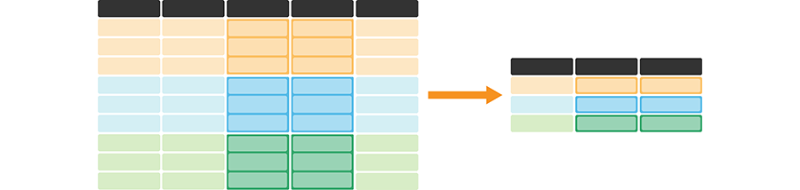
Figure 3.16: summarize and group_by is useful for calculating summary statistics on one or more column(s) for each group. It creates a new data frame—with one row for each group—containing the summary statistic(s) for each column being summarized. It also creates a column listing the value of the grouping variable. The darker, top row of each table represents the column headers. The orange, blue, and green colored rows correspond to the rows that belong to each of the three groups being represented in this cartoon example.
The group_by function takes at least two arguments. The first is the data
frame that will be grouped, and the second and onwards are columns to use in the
grouping. Here we use only one column for grouping (region), but more than one
can also be used. To do this, list additional columns separated by commas.
group_by(region_lang, region) |>
  summarize(
    min_most_at_home = min(most_at_home),
    max_most_at_home = max(most_at_home)
    )
## # A tibble: 35 × 3
## region min_most_at_home max_most_at_home
## <chr> <dbl> <dbl>
## 1 Abbotsford - Mission 0 137445
## 2 Barrie 0 182390
## 3 Belleville 0 97840
## 4 Brantford 0 124560
## 5 Calgary 0 1065070
## 6 Edmonton 0 1050410
## 7 Greater Sudbury 0 133960
## 8 Guelph 0 130950
## 9 Halifax 0 371215
## 10 Hamilton 0 630380
## # ℹ 25 more rowsNotice that group_by on its own doesn’t change the way the data looks.
In the output below, the grouped data set looks the same,
and it doesn’t appear to be grouped by region.
Instead, group_by simply changes how other functions work with the data,
as we saw with summarize above.
## # A tibble: 7,490 × 7
## # Groups:   region [35]
##    region   category language mother_tongue most_at_home most_at_work lang_known
##    <chr>    <chr>    <chr>            <dbl>        <dbl>        <dbl>      <dbl>
##  1 St. Joh… Aborigi… Aborigi…             5            0            0          0
##  2 Halifax  Aborigi… Aborigi…             5            0            0          0
##  3 Moncton  Aborigi… Aborigi…             0            0            0          0
##  4 Saint J… Aborigi… Aborigi…             0            0            0          0
##  5 Saguenay Aborigi… Aborigi…             5            5            0          0
##  6 Québec   Aborigi… Aborigi…             0            5            0         20
##  7 Sherbro… Aborigi… Aborigi…             0            0            0          0
##  8 Trois-R… Aborigi… Aborigi…             0            0            0          0
##  9 Montréal Aborigi… Aborigi…            30           15            0         10
## 10 Kingston Aborigi… Aborigi…             0            0            0          0
## # ℹ 7,480 more rows
3.9.4 Calculating summary statistics on many columns
Sometimes we need to summarize statistics across many columns.
An example of this is illustrated in Figure 3.17.
In such a case, using summarize alone means that we have to
type out the name of each column we want to summarize.
In this section we will meet two strategies for performing this task.
First we will see how we can do this using summarize + across.
Then we will also explore how we can use a more general iteration function,
map, to also accomplish this.
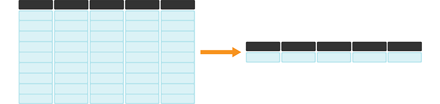
Figure 3.17: summarize + across or map is useful for efficiently calculating summary statistics on many columns at once. The darker, top row of each table represents the column headers.
summarize and across for calculating summary statistics on many columns
To summarize statistics across many columns, we can use the
summarize function we have just recently learned about.
However, in such a case, using summarize alone means that we have to
type out the name of each column we want to summarize.
To do this more efficiently, we can pair summarize with across
and use a colon : to specify a range of columns we would like
to perform the statistical summaries on.
Here we demonstrate finding the maximum value
of each of the numeric
columns of the region_lang data set.
## # A tibble: 1 × 4
##   mother_tongue most_at_home most_at_work lang_known
##           <dbl>        <dbl>        <dbl>      <dbl>
## 1       3061820      3836770      3218725    5600480
Note: Similar to when we use base R statistical summary functions (e.g.,
max,min,mean,sum, etc) withsummarizealone, the use of thesummarize+acrossfunctions paired with base R statistical summary functions also returnNAs when we apply them to columns that containNAs in the data frame.To resolve this issue, again we need to add the argument
na.rm = TRUE. But in this case we need to use it a little bit differently: we write a~, and then call the summary function with the first argument.xand the second argumentna.rm = TRUE. For example, for the previous example with themaxfunction, we would write## # A tibble: 1 × 4 ## mother_tongue most_at_home most_at_work lang_known ## <dbl> <dbl> <dbl> <dbl> ## 1 3061820 3836770 3218725 5600480The meaning of this unusual syntax is a bit beyond the scope of this book, but interested readers can look up anonymous functions in the
purrrpackage fromtidyverse.
map for calculating summary statistics on many columns
An alternative to summarize and across
for applying a function to many columns is the map family of functions.
Let’s again find the maximum value of each column of the
region_lang data frame, but using map with the max function this time.
map takes two arguments:
an object (a vector, data frame or list) that you want to apply the function to,
and the function that you would like to apply to each column.
Note that map does not have an argument
to specify which columns to apply the function to.
Therefore, we will use the select function before calling map
to choose the columns for which we want the maximum.
## $mother_tongue
## [1] 3061820
##
## $most_at_home
## [1] 3836770
##
## $most_at_work
## [1] 3218725
##
## $lang_known
## [1] 5600480Note: The
mapfunction comes from thepurrrpackage. But sincepurrris part of the tidyverse, once we calllibrary(tidyverse)we do not need to load thepurrrpackage separately.
The output looks a bit weird… we passed in a data frame, but the output doesn’t look like a data frame. As it so happens, it is not a data frame, but rather a plain list:
## [1] "list"So what do we do? Should we convert this to a data frame? We could, but a
simpler alternative is to just use a different map function. There
are quite a few to choose from, they all work similarly, but
their name reflects the type of output you want from the mapping operation.
Table 3.3 lists the commonly used map functions as well
as their output type.
map function |
Output |
|---|---|
map |
list |
map_lgl |
logical vector |
map_int |
integer vector |
map_dbl |
double vector |
map_chr |
character vector |
map_dfc |
data frame, combining column-wise |
map_dfr |
data frame, combining row-wise |
Let’s get the columns’ maximums again, but this time use the map_dfr function
to return the output as a data frame:
## # A tibble: 1 × 4
##   mother_tongue most_at_home most_at_work lang_known
##           <dbl>        <dbl>        <dbl>      <dbl>
## 1 3061820 3836770 3218725 5600480Note: Similar to when we use base R statistical summary functions (e.g.,
max,min,mean,sum, etc.) withsummarize,mapfunctions paired with base R statistical summary functions also returnNAvalues when we apply them to columns that containNAvalues.To avoid this, again we need to add the argument
na.rm = TRUE. When we use this withmap, we do this by adding a,and thenna.rm = TRUEafter specifying the function, as illustrated below:## # A tibble: 1 × 4 ## mother_tongue most_at_home most_at_work lang_known ## <dbl> <dbl> <dbl> <dbl> ## 1 3061820 3836770 3218725 5600480
The map functions are generally quite useful for solving many problems
involving repeatedly applying functions in R.
Additionally, their use is not limited to columns of a data frame;
map family functions can be used to apply functions to elements of a vector,
or a list, and even to lists of (nested!) data frames.
To learn more about the map functions, see the additional resources
section at the end of this chapter.
3.10 Apply functions across many columns with mutate and across
Sometimes we need to apply a function to many columns in a data frame. For example, we would need to do this when converting units of measurements across many columns. We illustrate such a data transformation in Figure 3.18.
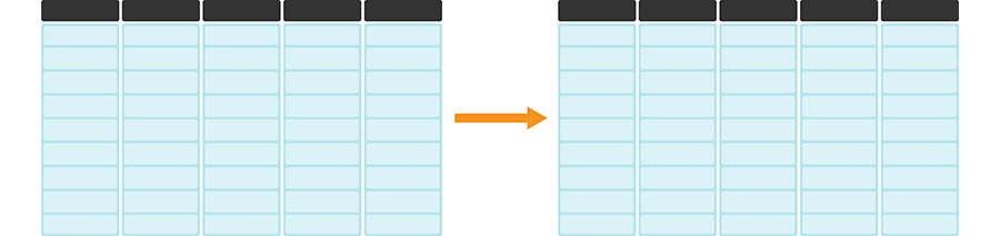
Figure 3.18: mutate and across is useful for applying functions across many columns. The darker, top row of each table represents the column headers.
For example,
imagine that we wanted to convert all the numeric columns
in the region_lang data frame from double type to integer type
using the as.integer function.
When we revisit the region_lang data frame,
we can see that this would be the columns from mother_tongue to lang_known.
## # A tibble: 7,490 × 7
##    region   category language mother_tongue most_at_home most_at_work lang_known
##    <chr>    <chr>    <chr>            <dbl>        <dbl>        <dbl>      <dbl>
##  1 St. Joh… Aborigi… Aborigi…             5            0            0          0
##  2 Halifax  Aborigi… Aborigi…             5            0            0          0
##  3 Moncton  Aborigi… Aborigi…             0            0            0          0
##  4 Saint J… Aborigi… Aborigi…             0            0            0          0
##  5 Saguenay Aborigi… Aborigi…             5            5            0          0
##  6 Québec   Aborigi… Aborigi…             0            5            0         20
##  7 Sherbro… Aborigi… Aborigi…             0            0            0          0
##  8 Trois-R… Aborigi… Aborigi…             0            0            0          0
##  9 Montréal Aborigi… Aborigi…            30           15            0         10
## 10 Kingston Aborigi… Aborigi…             0            0            0          0
## # ℹ 7,480 more rows
To accomplish such a task, we can use mutate paired with across.
This works in a similar way for column selection,
as we saw when we used summarize + across earlier.
As we did above,
we again use across to specify the columns using select syntax
as well as the function we want to apply on the specified columns.
However, a key difference here is that we are using mutate,
which means that we get back a data frame with the same number of columns and rows.
The only thing that changes is the transformation we applied
to the specified columns (here mother_tongue to lang_known).
## # A tibble: 7,490 × 7
##    region   category language mother_tongue most_at_home most_at_work lang_known
##    <chr>    <chr>    <chr>            <int>        <int>        <int>      <int>
##  1 St. Joh… Aborigi… Aborigi…             5            0            0          0
##  2 Halifax  Aborigi… Aborigi…             5            0            0          0
##  3 Moncton  Aborigi… Aborigi…             0            0            0          0
##  4 Saint J… Aborigi… Aborigi…             0            0            0          0
##  5 Saguenay Aborigi… Aborigi…             5            5            0          0
##  6 Québec   Aborigi… Aborigi…             0            5            0         20
##  7 Sherbro… Aborigi… Aborigi…             0            0            0          0
##  8 Trois-R… Aborigi… Aborigi…             0            0            0          0
##  9 Montréal Aborigi… Aborigi…            30           15            0         10
## 10 Kingston Aborigi… Aborigi…             0            0            0          0
## # ℹ 7,480 more rows
3.11 Apply functions across columns within one row with rowwise and mutate
What if you want to apply a function across columns but within one row? We illustrate such a data transformation in Figure 3.19.
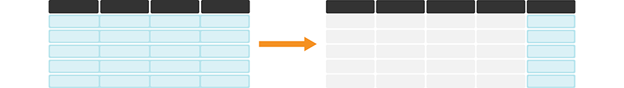
Figure 3.19: rowwise and mutate is useful for applying functions across columns within one row. The darker, top row of each table represents the column headers.
For instance, suppose we want to know the maximum value between mother_tongue,
most_at_home, most_at_work
and lang_known for each language and region
in the region_lang data set.
In other words, we want to apply the max function row-wise.
We will use the (aptly named) rowwise function in combination with mutate
to accomplish this task.
Before we apply rowwise, we will select only the count columns
so we can see all the columns in the data frame’s output easily in the book.
So for this demonstration, the data set we are operating on looks like this:
## # A tibble: 7,490 × 4
## mother_tongue most_at_home most_at_work lang_known
## <dbl> <dbl> <dbl> <dbl>
## 1 5 0 0 0
## 2 5 0 0 0
## 3 0 0 0 0
## 4 0 0 0 0
## 5 5 5 0 0
## 6 0 5 0 20
## 7 0 0 0 0
## 8 0 0 0 0
## 9 30 15 0 10
## 10 0 0 0 0
## # ℹ 7,480 more rowsNow we apply rowwise before mutate, to tell R that we would like
the mutate function to be applied across, and within, a row,
as opposed to being applied on a column
(which is the default behavior of mutate):
region_lang |>
select(mother_tongue:lang_known) |>
rowwise() |>
mutate(maximum = max(c(mother_tongue,
most_at_home,
most_at_work,
lang_known)))## # A tibble: 7,490 × 5
## # Rowwise:
## mother_tongue most_at_home most_at_work lang_known maximum
## <dbl> <dbl> <dbl> <dbl> <dbl>
## 1 5 0 0 0 5
## 2 5 0 0 0 5
## 3 0 0 0 0 0
## 4 0 0 0 0 0
## 5 5 5 0 0 5
## 6 0 5 0 20 20
## 7 0 0 0 0 0
## 8 0 0 0 0 0
## 9 30 15 0 10 30
## 10 0 0 0 0 0
## # ℹ 7,480 more rowsWe see that we get an additional column added to the data frame,
named maximum, which is the maximum value between mother_tongue,
most_at_home, most_at_work and lang_known for each language
and region.
Similar to group_by,
rowwise doesn’t appear to do anything when it is called by itself.
However, we can apply rowwise in combination
with other functions to change how these other functions operate on the data.
Notice if we used mutate without rowwise,
we would have computed the maximum value across all rows
rather than the maximum value for each row.
Below we show what would have happened had we not used
rowwise. In particular, the same maximum value is reported
in every single row; this code does not provide the desired result.
region_lang |>
  select(mother_tongue:lang_known) |>
  mutate(maximum = max(c(mother_tongue,
                         most_at_home,
                         most_at_home,
                         lang_known)))
## # A tibble: 7,490 × 5
## mother_tongue most_at_home most_at_work lang_known maximum
## <dbl> <dbl> <dbl> <dbl> <dbl>
## 1 5 0 0 0 5600480
## 2 5 0 0 0 5600480
## 3 0 0 0 0 5600480
## 4 0 0 0 0 5600480
## 5 5 5 0 0 5600480
## 6 0 5 0 20 5600480
## 7 0 0 0 0 5600480
## 8 0 0 0 0 5600480
## 9 30 15 0 10 5600480
## 10 0 0 0 0 5600480
## # ℹ 7,480 more rows3.12 Summary
Cleaning and wrangling data can be a very time-consuming process. However, it is a critical step in any data analysis. We have explored many different functions for cleaning and wrangling data into a tidy format. Table 3.4 summarizes some of the key wrangling functions we learned in this chapter. In the following chapters, you will learn how you can take this tidy data and do so much more with it to answer your burning data science questions!
| Function | Description |
|---|---|
across |
allows you to apply function(s) to multiple columns |
filter |
subsets rows of a data frame |
group_by |
allows you to apply function(s) to groups of rows |
mutate |
adds or modifies columns in a data frame |
map |
general iteration function |
pivot_longer |
generally makes the data frame longer and narrower |
pivot_wider |
generally makes a data frame wider and decreases the number of rows |
rowwise |
applies functions across columns within one row |
separate |
splits up a character column into multiple columns |
select |
subsets columns of a data frame |
summarize |
calculates summaries of inputs |
3.13 Exercises
Practice exercises for the material covered in this chapter can be found in the accompanying worksheets repository in the “Cleaning and wrangling data” row. You can launch an interactive version of the worksheet in your browser by clicking the “launch binder” button. You can also preview a non-interactive version of the worksheet by clicking “view worksheet.” If you instead decide to download the worksheet and run it on your own machine, make sure to follow the instructions for computer setup found in Chapter 13. This will ensure that the automated feedback and guidance that the worksheets provide will function as intended.
3.14 Additional resources
- As we mentioned earlier,
tidyverseis actually an R meta package: it installs and loads a collection of R packages that all follow the tidy data philosophy we discussed above. One of thetidyversepackages isdplyr—a data wrangling workhorse. You have already met many ofdplyr’s functions (select,filter,mutate,arrange,summarize, andgroup_by). To learn more about these functions and meet a few more useful functions, we recommend you check out Chapters 5-9 of the STAT545 online notes. of the data wrangling, exploration, and analysis with R book. - The
dplyrR package documentation (Wickham, François, et al. 2021) is another resource to learn more about the functions in this chapter, the full set of arguments you can use, and other related functions. The site also provides a very nice cheat sheet that summarizes many of the data wrangling functions from this chapter. - Check out the
tidyselectR package page (Henry and Wickham 2021) for a comprehensive list ofselecthelpers. These helpers can be used to choose columns in a data frame when paired with theselectfunction (and other functions that use thetidyselectsyntax, such aspivot_longer). The documentation forselecthelpers is a useful reference to find the helper you need for your particular problem. - R for Data Science (Wickham and Grolemund 2016) has a few chapters related to
data wrangling that go into more depth than this book. For example, the
tidy data chapter covers tidy data,
pivot_longer/pivot_widerandseparate, but also covers missing values and additional wrangling functions (likeunite). The data transformation chapter coversselect,filter,arrange,mutate, andsummarize. And themapfunctions chapter provides more about themapfunctions. - You will occasionally encounter a case where you need to iterate over items in a data frame, but none of the above functions are flexible enough to do what you want. In that case, you may consider using a for loop.