Appendix - Defining functions

Appendix - Defining functions#

Defining functions in R:#

In this course, we will get to practice writing functions (and then testing them) in the R programming language. Given this has not been covered in the course pre-requisites, we will cover it here briefly. To learn more about functions in R, we refer you to the functions chapter in the Advanced R book.

Use variable <- function(…arguments…) { …body… } to create a function and give it a name

Example:

add_two_numbers <- function(x, y) {
  x + y
}

add_two_numbers(1, 4)

5

Functions in R are objects. This is referred to as “first-class functions”.
The last line of the function returns the object created, or listed there. To return a value early use the special word return (as shown below).

math_two_numbers <- function(x, y, operation) {
  if (operation == "add") {
    return(x + y)
  } 
  x - y
}

math_two_numbers (1, 4, "add")

5

math_two_numbers (1, 4, "subtract")

-3

Default function arguments#

Default values can be specified in the function definition:

math_two_numbers <- function(x, y, operation = "add") {
  if (operation == "add") {
    return(x + y)
  } 
  x - y
}

math_two_numbers (1, 4)

5

math_two_numbers (1, 4, "subtract")

-3

Optional - Advanced#

Extra arguments via `...`#

If we want our function to be able to take extra arguments that we don’t specify, we must explicitly convert ... to a list (otherwise ... will just return the first object passed to ...):

add <- function(x, y, ...) {
    print(list(...))
}
add(1, 3, 5, 6)

[[1]]
[1] 5

[[2]]
[1] 6

Lexical scoping in R#

R’s lexical scoping follows several rules, we will cover the following 3:

Name masking
Dynamic lookup
A fresh start

Name masking#

Object names which are defined inside a function mask object names defined outside of that function. For example, below x is first defined in the global environment, and then also defined in the function environment. x in the function environment masks x in the global environment, so the value of 5 is used in to_add + x instead of 10:

x <- 10

add_to_x <- function(to_add) {
    x <- 5
    to_add + x
}

add_to_x(2)

7

If a function refers to an object name that is not defined inside the function, then R looks at the environment one level above. And if it is not found there, it again, looks another level above. This will happen all the way up the environment tree until it searches all possible environments for that session (including the global environment and loaded packages).

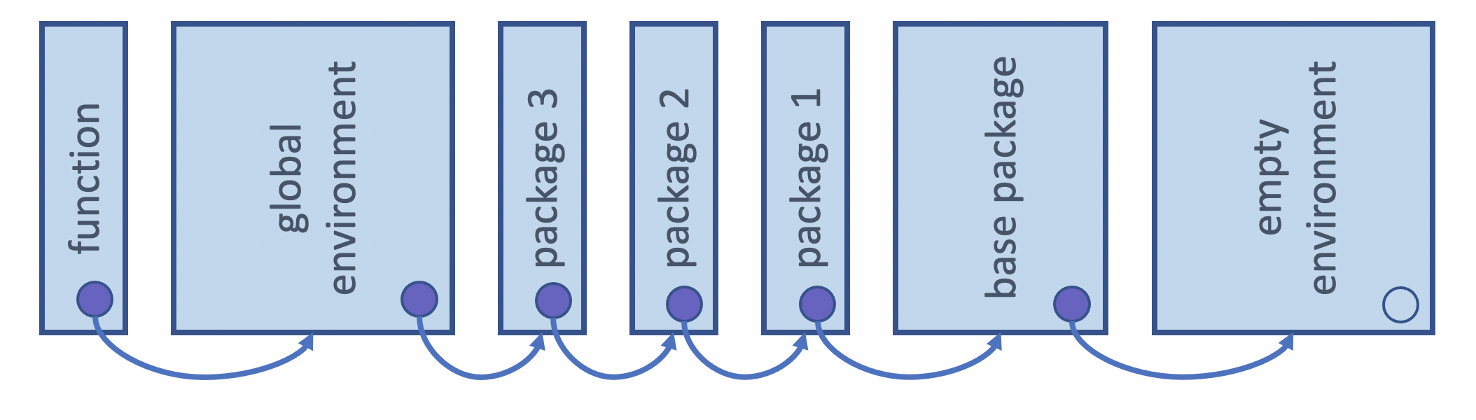
Attribution: Derived from Advanced R by Hadley Wickham

Here x is not defined in the function environment, and so R then looks one-level up to the global environment to try to find x. In this case it does and it is then used to calculate to_add + x:

x <- 10

add_to_x <- function(to_add) {
    to_add + x
}

add_to_x(2)

12

Dynamic lookup#

R does not look up the values for objects it references when it is defined/created, instead it does this when the function is called. This can lead to the function returning different things depending on the values of the objects it references outside of the function’s environment.

For example, each time the function add_to_x is run, R looks up the current value of x and uses that to compute to_add + x:

add_to_x <- function(to_add) {
    to_add + x
}

x <- 10
add_to_x(2)

x <- 20
add_to_x(2)

12

22

A fresh start#

Functions in R have no memory of what happened the last time they were called. This happens because a new function environment is created, R created a new environment in which to execute it.

For example, even though we update the value of x inside the function by adding two to it every time we execute it, it returns the same value each time, because R creates a new function environment each time we run it and that environment has no recollection of what happened the last time the function was run:

x <- 10

add_to_x <- function(to_add) {
    x <- to_add + x
    x
}

add_to_x(2)
add_to_x(2)
add_to_x(2)

12

Lazy evaluation#

In R, function arguments are lazily evaluated: they’re only evaluated if accessed.

Knowing that, now consider the add_one function written in both R and Python below:

# R code (this would work)
add_one <- function(x, y) {
    x <- x + 1
    return(x)
} 

# Python code (this would not work)
def add_one(x, y):
    x = x + 1
    return x

Why will the above add_one function will work in R, but the equivalent version of the function in python would break?

Python evaluates the function arguments before it evaluates the function and because it doesn’t know what y is, it will break even though it is not used in the function.
R performs lazy evaluation, meaning it delays the evaluation of the function arguments until its value is needed within/inside the function. Since y is never referenced inside the function, R doesn’t complain, or even notice it.

`add_one` in R#

add_one <- function(x, y) {
    x <- x + 1
    return(x)
} 

This works:

add_one(2, 1)

and so does this:

add_one(2)

`add_one` in Python#

def add_one(x, y):
    x = x + 1
    return x`

This works:

add_one(2, 1)

This does not:

add_one(2)

---------------------------------------------------------------------------
TypeError                                 Traceback (most recent call last)
<ipython-input-5-f2e542671748> in <module>
----> 1 add_one(2)

TypeError: add_one() missing 1 required positional argument: 'y'

The power of lazy evaluation#

Let’s you have easy to use interactive code like this:

dplyr::select(mtcars, mpg, cyl, hp, qsec)

A data.frame: 32 × 4
	mpg	cyl	hp	qsec
	<dbl>	<dbl>	<dbl>	<dbl>
Mazda RX4	21.0	6	110	16.46
Mazda RX4 Wag	21.0	6	110	17.02
Datsun 710	22.8	4	93	18.61
Hornet 4 Drive	21.4	6	110	19.44
Hornet Sportabout	18.7	8	175	17.02
Valiant	18.1	6	105	20.22
Duster 360	14.3	8	245	15.84
Merc 240D	24.4	4	62	20.00
Merc 230	22.8	4	95	22.90
Merc 280	19.2	6	123	18.30
Merc 280C	17.8	6	123	18.90
Merc 450SE	16.4	8	180	17.40
Merc 450SL	17.3	8	180	17.60
Merc 450SLC	15.2	8	180	18.00
Cadillac Fleetwood	10.4	8	205	17.98
Lincoln Continental	10.4	8	215	17.82
Chrysler Imperial	14.7	8	230	17.42
Fiat 128	32.4	4	66	19.47
Honda Civic	30.4	4	52	18.52
Toyota Corolla	33.9	4	65	19.90
Toyota Corona	21.5	4	97	20.01
Dodge Challenger	15.5	8	150	16.87
AMC Javelin	15.2	8	150	17.30
Camaro Z28	13.3	8	245	15.41
Pontiac Firebird	19.2	8	175	17.05
Fiat X1-9	27.3	4	66	18.90
Porsche 914-2	26.0	4	91	16.70
Lotus Europa	30.4	4	113	16.90
Ford Pantera L	15.8	8	264	14.50
Ferrari Dino	19.7	6	175	15.50
Maserati Bora	15.0	8	335	14.60
Volvo 142E	21.4	4	109	18.60

Notes:

There’s more than just lazy evaluation happening in the code above, but lazy evaluation is part of it.
package::function() is a way to use a function from an R package without loading the entire library.

Exception handling#

Sometimes our code is correct but we still encounter errors. This commonly occurs with functions when users attempt to use them in weird and creative ways that the developer did not intend. Developers are well advised to try to anticipate some of this user behaviour and guard against this in a way that can be of help to the user. One way to do this is to have a function fail intentionally when incorrect user input is given.

Imagine we have a simple function to convert temperatures from Fahrenheit to Celsius:

fahr_to_celsius <- function(temp) {
  (temp - 32) * 5/9
}

What if our user anticipates that our function can handle numbers written as strings? When this happens our users gets a somewhat cryptic error message (which is inversely correlated with their knowledge of the R programming language):

fahr_to_celsius("thirty")

Error in temp - 32: non-numeric argument to binary operator
Traceback:

1. fahr_to_celsius("thirty")

This error message is not as helpful as it could be! Also, if this calculation happened to take a long time, it might be nicer to check the data type before we attempt the calculation and then if the wrong data type was given, throw an purposeful error with a more helpful error message. One way we can do this simply in R is using a conditional (i.e., if statement) to test the type and then calling stop with a useful error message if the type is incorrect.

For example with the fahr_to_celsius function, we can use if(!is.numeric(temp)) to check whether temp is not numeric. And then if it is not, stop causes a break and the printing out of the more helpful error message “fahr_to_celsius expects a vector of numeric values

fahr_to_celsius <- function(temp) {
  if(!is.numeric(temp)) {    
    stop("`fahr_to_celsius` expects a vector of numeric values")
  }
  (temp - 32) * 5/9
}

fahr_to_celsius("thirty")

Error in fahr_to_celsius("thirty"): `fahr_to_celsius` expects a vector of numeric values
Traceback:

1. fahr_to_celsius("thirty")
2. stop("`fahr_to_celsius` expects a vector of numeric values")   # at line 3 of file <text>

If you wanted to issue a warning instead of an error, you could use warning in place of stop in the example above. However, in most cases it is better practice to throw an error than to print a warning…

More advanced exception handling exists in R, and I invite interested learner to read more about it here in the Condition Handling and Defensive Programming sections of Advanced R.

Programming with the `tidyverse` functions#

The functions from the tidyverse are beautiful to use interactively - with these functions, we can “pretend” that the data frame column names are objects in the global environment and refer to them without quotations (e.g., "")

library(tidyverse)
library(gapminder)

gapminder |>
  filter(country == "Canada", year == 1952)

── Attaching core tidyverse packages ──────────────────────── tidyverse 2.0.0 ──
✔ dplyr     1.1.2     ✔ readr     2.1.4
✔ forcats   1.0.0     ✔ stringr   1.5.0
✔ ggplot2   3.4.3     ✔ tibble    3.2.1
✔ lubridate 1.9.2     ✔ tidyr     1.3.0
✔ purrr     1.0.2     

── Conflicts ────────────────────────────────────────── tidyverse_conflicts() ──
✖ dplyr::filter() masks stats::filter()
✖ dplyr::lag()    masks stats::lag()
ℹ Use the conflicted package (<http://conflicted.r-lib.org/>) to force all conflicts to become errors

A tibble: 1 × 6
country	continent	year	lifeExp	pop	gdpPercap
<fct>	<fct>	<int>	<dbl>	<int>	<dbl>
Canada	Americas	1952	68.75	14785584	11367.16

expecially when compared with base R:

gapminder[gapminder$country == "Canada" & gapminder$year == 1952, ]

A tibble: 1 × 6
country	continent	year	lifeExp	pop	gdpPercap
<fct>	<fct>	<int>	<dbl>	<int>	<dbl>
Canada	Americas	1952	68.75	14785584	11367.16

However, the beauty of being able to refer to data frame column names in R without quotations, leads to problems when we try to use them in a function. For example,

filter_gap <- function(col, val) {
    filter(gapminder, col == val)
}

filter_gap(country, "Canada")

Error: object 'country' not found
Traceback:

1. filter_gap(country, "Canada")
2. filter(gapminder, col == val)   # at line 4 of file <text>
3. filter.tbl_df(gapminder, col == val)
4. filter_impl(.data, quo)

Why does filter work with non-quoted variable names, but our function filter_gap fail? At a very high-level, this is because filter is doing more behind the scenes to handle these unquoted column names than we see without looking at the source code. So to make this work for our function, we need to do a little more work too.

Given that this is not a course in R programming, we will not go into the details of why this happens, but we will show one way of how to handle this. For learners intersted to learn more about why this happens, we recommend reading these two resources:

Defining `tidyverse` functions by embracing column names: `{{ }}`#

In the newest release of the rlang R package, there has been the introduction of the {{ (pronounced “curly curly”) operator. This operator does the necessary work behind the scenes so that you can continue to use unquoted column names with the tidyverse functions even when you use them in functions that you write yourself.

To use the {{ operator, we “embrace” the unquoted column names when we refer to them inside our function body. An important note is that there are several ways to implement the usage of unquoted column names in R, and the {{ operator only works with the tidyverse functions. Please refer to the Metaprogramming chapter of Advanced R if you need to do this with non-tidyverse functions.

Here’s the function we show above working when we use the {{ operator to “embrace” the unquoted column names:

filter_gap <- function(col, val) {
  filter(gapminder, {{col}} == val)
}

filter_gap(country, "Canada")

A tibble: 12 × 6
country	continent	year	lifeExp	pop	gdpPercap
<fct>	<fct>	<int>	<dbl>	<int>	<dbl>
Canada	Americas	1952	68.750	14785584	11367.16
Canada	Americas	1957	69.960	17010154	12489.95
Canada	Americas	1962	71.300	18985849	13462.49
Canada	Americas	1967	72.130	20819767	16076.59
Canada	Americas	1972	72.880	22284500	18970.57
Canada	Americas	1977	74.210	23796400	22090.88
Canada	Americas	1982	75.760	25201900	22898.79
Canada	Americas	1987	76.860	26549700	26626.52
Canada	Americas	1992	77.950	28523502	26342.88
Canada	Americas	1997	78.610	30305843	28954.93
Canada	Americas	2002	79.770	31902268	33328.97
Canada	Americas	2007	80.653	33390141	36319.24

The walrus operator `:=` is needed when assigning values#

For similar reasons, the walrus operator (:=) is needed when writing functions that create new columns using unquoted column names with the tidyverse functions:

group_summary <- function(data, group, col, fun) {
  data |>
    group_by({{ group }}) |>
    summarise( {{ col }} := fun({{ col }}))
}

group_summary(gapminder, continent, gdpPercap, mean)

A tibble: 5 × 2
continent	gdpPercap
<fct>	<dbl>
Africa	2193.755
Americas	7136.110
Asia	7902.150
Europe	14469.476
Oceania	18621.609

Function documentation#

Function documentation is extremely useful at both the time of function creation/development, as well as at the time of function usage by the user. At the time of creation/development, it is useful for clearly delineating and communication the planned function’s specifications. At the time of usage, it is often the primary documentation a user will refer to in order to understand how to use the function. If a function is not well documented, it will not be well understood or widely used.

Function documentation in R#

In R, we write function documentation in a style that the roxygen2 R package can use to automatically generate nicely formatted documentation, accessible via R’s help function, when we create R packages. This is not available to us until we package our functions in software packages, however it is a good practice to get into because it helps ensure you document the key aspects of a function for your user, and it means that when you go to create an R package to share your function, you will have already correctly formatted the function documentation - saving future you some work!

#' Converts temperatures from Fahrenheit to Celsius.
#'    
#' @param temp a vector of temperatures in Fahrenheit
#' 
#' @return a vector of temperatures in Celsius
#' 
#' @examples
#' fahr_to_celcius(-20)
fahr_to_celsius <- function(temp) {
    (temp - 32) * 5/9
}

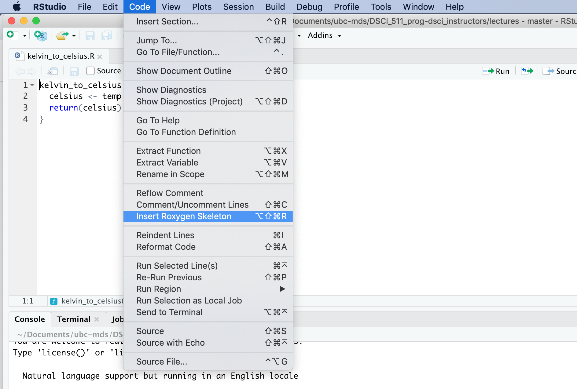
RStudio has a nice feature to provide a roxygen2 formatted skeleton for function documentation. To use it, you put the cursor in the function definition, and then select the menu items “Code” > “Insert Roxygen Skeleton”:

Practice writing functions in R#

To practice writing functions in R, you can attempt this worksheet: https://github.com/UBC-DSCI/dsci-310-student/blob/main/practice/worksheet_functions_in_r.ipynb

Note: to access the automated software tests for feedback on your answers, you will want to clone or download this GitHub repo and navigate to the practice directory.

Defining functions in Python#

In this course, we will get to practice writing functions (and then testing them) in the Python programming language. We will only cover it here briefly. To learn more about functions in Python, we refer you to the Module 6: Functions Fundamentals and Best Practices from the Programming in Python for Data Science course.

Functions in Python are defined using the reserved word def. A colon follows the function arguments to indicate where the function body should starte. White space, in particular indentation, is used to indicate which code belongs in the function body and which does not. A general form for fucntion definition is shown below:

def function_name(…function arguments…):
    …function body…

Here’s a working example:

add_two_numbers <- function(x, y) {
  x + y
}

add_two_numbers(1, 4)

5

Functions in R are objects. This is referred to as “first-class functions”.
The last line of the function returns the object created, or listed there. To return a value early use the special word return (as shown below).

math_two_numbers <- function(x, y, operation) {
  if (operation == "add") {
    return(x + y)
  } 
  x - y
}

math_two_numbers (1, 4, "add")

5

math_two_numbers (1, 4, "subtract")

-3

Default function arguments#

Default values can be specified in the function definition:

math_two_numbers <- function(x, y, operation = "add") {
  if (operation == "add") {
    return(x + y)
  } 
  x - y
}

math_two_numbers (1, 4)

5

math_two_numbers (1, 4, "subtract")

-3

Optional - Advanced#

Extra arguments via `...`#

If we want our function to be able to take extra arguments that we don’t specify, we must explicitly convert ... to a list (otherwise ... will just return the first object passed to ...):

Appendix - Defining functions

Contents

Appendix - Defining functions#

Defining functions in R:#

Default function arguments#

Optional - Advanced#

Extra arguments via ...#

Lexical scoping in R#

Name masking#

Dynamic lookup#

A fresh start#

Lazy evaluation#

add_one in R#

add_one in Python#

The power of lazy evaluation#

Exception handling#

Programming with the tidyverse functions#

Defining tidyverse functions by embracing column names: {{ }}#

The walrus operator := is needed when assigning values#

Function documentation#

Function documentation in R#

Practice writing functions in R#

Defining functions in Python#

Default function arguments#

Optional - Advanced#

Extra arguments via ...#

Extra arguments via `...`#

`add_one` in R#

`add_one` in Python#

Programming with the `tidyverse` functions#

Defining `tidyverse` functions by embracing column names: `{{ }}`#

The walrus operator `:=` is needed when assigning values#

Extra arguments via `...`#