Jupyter Book¶

1. Introduction¶

I’m Tom. Nice to meet you!¶

Fig. 29 This is me!¶

I’m a postdoc with the UBC Master of Data Science. I have a background in Civil Engineering / Climate Science & PhD in Coastal Engineering (topic: Using machine learning for predicting coastal storm erosion). Strong Python / intermediate R.

1.1. Jupyter Book¶

Fig. 30 The Jupyter Book logo.¶

Jupyter Book is an open-source project for building books and documents from standard computational and data science materials such as Jupyter Notebooks and Markdown documents.

In fact, this website is built with Jupyter Book!

In this session, I’ll go through an example of creating a Jupyter Book from scratch and some of the key features Jupyter Book offers. If you’re interested in using Jupyter Book and learning more, check out the excellent official Jupyter Book documentation.

1.2. Key Jupyter Book Features¶

Write publication-quality content including figures, math, citations & cross-references!
Write content as Jupyter Notebooks, markdown, or reStructuredText
Add interactivity to your book, e.g., toggle visibility of cells, connect with an online service like Binder, and include interactive outputs (e.g., figures and widgets).
Generate a variety of outputs, including websites (HTML, CSS, JS), markdown and PDF.
A command-line interface to quickly build books, e.g., jupyter-book build mybook/

Note

Read more in the official Jupyter Book documentation.

1.3 Key Jupyter Book Information¶

Jupyter Book is part of the Executable Book Project, an “international collaboration to build open source tools that facilitate publishing computational narratives using the Jupyter ecosystem”.
Jupyter Book uses the Sphinx documentation tool.
Jupyter Book is currently at v0.7.4 and is actively being developed, there may be some breaking backward compatibility API changes prior to the v1.0.0 release.
There is a growing community contributing to and discussing Jupyter Book: check out the GitHub Issues page for the latest discussions and developments.

2. Jupyter Book Tutorial¶

In this workshop we are going to build our very own Jupyter Book, containing text, images and code related to our favourite planet - Jupiter!

Let’s take a look at that book now: http://www.tomasbeuzen.com/my-jupiter-book/

If you want to follow this tutorial on your own machine, you’ll need the following:

Python (recommended: install the miniconda distribution)
GitHub account
Linux/MacOS (Jupyter Book on Windows is an active area of development)

Attention

A note from Phil Austin, who is actively working on Windows integration:

The “Working on Windows” documentation I wrote at the beginning of the summer is completely out of date. Windows is very close to parity with unix now. If anyone needs to make a jupyter-book on windows, the extra steps after installing would be to upgrade jupyter-book using this PR and use the current master for jupyter-sphinx.

3. Installing Jupyter Book¶

The first thing we need to do is install Jupyter Book. I highly recommend you do this in a virtual environment. I use conda to manage my virtual environments - if you’re interested in doing the same, I recommend installing the miniconda distribution.

You can create and activate a new environment with conda using the command line:

$ conda create -n jupydays python=3.8 -y
$ conda activate jupydays

Note

Note that we are naming our environment “jdays” here but you can call it anything you like.

Now it’s time to install Jupyter Book. We’ll also need the Pandas, Plotly and sphinx-thebe libraries so we’ll install those too:

pip install jupyter-book pandas plotly sphinx-thebe

4. Creating a Book Structure¶

Jupyter Book comes with a CL tool that allows you to quickly create and build books. To create the skeleton of our book, type the following at the command line:

jupyter-book create jupiter

Note

Here we are calling our book “jupiter”, but you can choose to call your book anything you like.

Tip

You can also use the short-hand jb for jupyter-book, e.g., jb build jupiter.

You will now have a new directory called jupiter (or whatever you chose to call your book), with the following contents:

jupiter
  ├── _config.yml
  ├── _toc.yml
  ├── content.md
  ├── intro.md
  ├── markdown.md
  ├── notebooks.ipynb
  ├── references.bib
  └── requirements.txt

5. Adding Content¶

5.1. Re-structuring Our Book Directory¶

Jupyter Book supports a number of file types:

Markdown (.md)
Notebooks (.ipynb)
etc.

As Markdown and Jupyter Notebooks will likely be the most common file types you will use, I’ll show an example of them here.

We’ll start from scratch, so go ahead and delete the following starter files in your book directory:

content.md
intro.md
markdown.md
notebooks.ipynb

rm content.md intro.md markdown.md notebooks.ipynb

5.2. Adding a Markdown Content File¶

Let’s start our book by adding a markdown file. Open up your new book in an editor of your choice (I recommend JupyterLab as we’ll be adding a Jupyter Notebook in the next section) and create a new markdown file named introduction.md.

We’ll use this file as a demonstration of some of the main types of content you can add to a Jupyter Book.

5.2.1. Markdown Text¶

We’ll start by adding some simple Markdown text to our file. If you are not familiar with markdown syntax, check out this cheat sheet. You can copy-paste the following content directly into your introduction.md file.

# Jupiter Book

This book contains information about the planet **Jupiter** - the fifth planet from the sun and the largest planet in the solar system!

Before we take a look at how our book renders with this text, let’s add an image too.

5.2.2. Figures¶

You can include figures in your Jupyter Book using the following syntax:

```{figure} my_image.png
---
height: 150px
name: my-image
---
Here is my image's caption!
```

While your image can be contained and referenced to from your book’s root directory, you can also include images via urls. Let’s include an image of the planet Jupiter in our introduction.md file using the following:

```{figure} https://solarsystem.nasa.gov/system/resources/detail_files/2486_stsci-h-p1936a_1800.jpg
---
height: 300px
name: jupiter-figure
---
The beautiful planet Jupiter!
```

The reason we give our image a “name” is so that we can easily reference it with the syntax:

{numref}`jupiter-figure`

Let’s add a sentence including a reference to our figure to demonstrate this. The full file should now look like this:

# Jupiter Book

This book contains information about the planet Jupiter - the fifth planet from the sun and the largest planet in the solar system! {numref}`jupiter-figure` below shows an image of Jupiter captured by the Hubble Space Telescope on June 27, 2019.

```{figure} https://solarsystem.nasa.gov/system/resources/detail_files/2486_stsci-h-p1936a_1800.jpg
---
height: 300px
name: jupiter-figure
---
The beautiful planet Jupiter! Source: [NASA](https://solarsystem.nasa.gov/resources/2486/hubbles-new-portrait-of-jupiter/?category=planets_jupiter).
```

At this point, we should probably build our book to make sure it’s looking as expected. To do that we first need to modify our _toc.yml file. This file contains the table of contents of our book. Open that file now and remove everything in there. Then simply add the following:

- file: introduction

Note

There are a number of ways you can configure your table of contents, e.g., with Headers, Sub-headers, Chapters, Section, etc, that I won’t go into here because it is all very well explained in the official Jupyter Book documentation!

We can now build our book from the command line by making sure that we are in our book’s root directory and then using:

$ jb build ./

Warning

You may get some red warnings printed to your output as the book is built, but these are typically just warnings or suggestions for how to improve your book.

Once the build is finished you’ll have a new sub-directory called _build/html in your book’s root, navigate to that location and open up _build/html/index.html. It should look something like this:

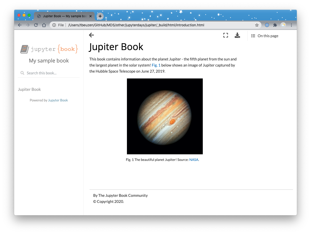
Fig. 31 First build of our Jupiter book.¶

5.2.3. Math and Equations¶

Jupyter Book uses MathJax for typesetting math which allows you to add LaTeX-style maths to your book. You can add inline maths, math blocks and numbered equations to your Jupyter Book. Let’s go ahead and create a new heading in our introduction.md file that includes some maths.

Inline math can be defined using $ as follows:

Jupiter has a mass of:  $m_{j} \approx 1.9 \times 10^{27} kg$

Jupiter has a mass of: $m_{j} \approx 1.9 \times 10^{27} kg$

Math blocks can be defined using $$ notation:

$$
  m_{j} \approx 1.9 \times 10^{27} kg
$$

\[ m_{j} \approx 1.9 \times 10^{27} kg \]

Note

If you prefer, math blocks can also be defined with \begin{equation} and \begin{equation} instead of $$.

Numbered equations can be defined like this (this is the style I recommend you use most often):

```{math}
:label: my_label
m_{j} \approx 1.9 \times 10^{27} kg
```

(1)¶\[m_{j} \approx 1.9 \times 10^{27} kg\]

Let’s add some more content to our Jupiter book. Copy and append the following text to your introduction.md file:

## The Mass of Jupiter

We can estimate the mass of Jupiter from the period and size of an object orbiting it. For example, we can use Jupiter's moon Callisto to estimate it's mass.

Callisto's period: $p_{c}=16.7 days$

Callisto's orbit radius: $r_{c}=1,900,000 km$

Now, using [Kepler's Law](https://solarsystem.nasa.gov/resources/310/orbits-and-keplers-laws/) we can work out the mass of Jupiter.

```{math}
:label: eq1
m_{j} \approx \frac{r_{c}}{p_{c}} \times 7.9 \times 10^{10}
```

```{math}
:label: eq2
m_{j} \approx 1.9 \times 10^{27} kg
```

You can then re-build your book (jb build ./) and open _build/html/index.html to make sure everything is rendering as expected.

5.2.4. Controlling the Page Layout¶

There are a number of different ways you can control the layout of your Jupyter Book pages which are described in detail in the official Jupyter Book docs. The layout change I use most often is adding content to a margin on my page. You can add a margin using the following directive:

```{margin} An optional title
Some margin content.
```

Let’s add some margin content to our book now:

```{margin} Did you know?
Jupiter is 11.0x larger than Earth!
```

5.2.5. Admonitions¶

You may have noticed that I enjoy adding admonitions to my books - they can be used to break up your book’s content and draw attention to important information. There are all sorts of different admonitions you can use in Jupyter Book which are listed here in the Jupyter Book documentation. Admonitions are created with the syntax:

```{note}
I am a useful note!
```

Here are a few examples:

Note

I am a useful note!

Tip

I am a helpful tip!

Warning

I am a dire warning!

Feel free to add the following admonition to introduction.md:

```{hint}
NASA provides a lot more information about the physical characteristics of Jupiter [here](https://solarsystem.nasa.gov/planets/jupiter/by-the-numbers/).
```

5.2.6. Citations and a Bibliography¶

The last piece of content I want to show you is adding references and a bibliography to your book. You can add citations of any works stored in the references.bib bibtex file that is located in your book’s root directory.

To include a citation in your book, add a bibtex entry to references.bib, for example:

---
---

@article{mayor1995jupiter,
    title={A Jupiter-mass companion to a solar-type star},
    author={Mayor, Michel and Queloz, Didier},
    journal={Nature},
    volume={378},
    number={6555},
    pages={355--359},
    year={1995},
    publisher={Nature Publishing Group}
}

@article{guillot1999interiors,
    title={Interiors of giant planets inside and outside the solar system},
    author={Guillot, Tristan},
    journal={Science},
    volume={286},
    number={5437},
    pages={72--77},
    year={1999},
    publisher={American Association for the Advancement of Science}
}

Hint

See the BibTex documentation for information about the BibTex reference style. Google Scholar facilitates exporting a bibtex citation format.

You can then reference the work in your Jupyter Book using the following directive:

{cite}`mayor1995jupiter`

Or for multiple citations:

{cite}`mayor1995jupiter,guillot1999interiors`

You can then create a bibliography from references.bib using:

```{bibliography} references.bib
```

For example, try adding this to your introduction.md file:

There might even be more planets out there with a similar mass to Jupiter {cite}`mayor1995jupiter,guillot1999interiors`!

## Bibliography

```{bibliography} references.bib
```

Your final introduction.md file should look something like this:

# Jupiter Book

This book contains information about the planet Jupiter - the fifth planet from the sun and the largest planet in the solar system! {numref}`jupiter-figure` below shows an image of Jupiter captured by the Hubble Space Telescope on June 27, 2019.

```{figure} https://solarsystem.nasa.gov/system/resources/detail_files/2486_stsci-h-p1936a_1800.jpg
---
height: 300px
name: jupiter-figure
---
The beautiful planet Jupiter! Source: [NASA](https://solarsystem.nasa.gov/resources/2486/hubbles-new-portrait-of-jupiter/?category=planets_jupiter).
```

## The Mass of Jupiter

We can estimate the mass of Jupiter from the period and size of an object orbiting it. For example, we can use Jupiter's moon Callisto to estimate it's mass.

Callisto's period: $p_{c}=16.7 days$

Callisto's orbit radius: $r_{c}=1,900,000 km$

Now, using [Kepler's Law](https://solarsystem.nasa.gov/resources/310/orbits-and-keplers-laws/) we can work out the mass of Jupiter.

```{math}
:label: eq1
m_{j} \approx \frac{r_{c}}{p_{c}} \times 7.9 \times 10^{10}
```

```{math}
:label: eq2
m_{j} \approx 1.9 \times 10^{27} kg
```

```{margin} Did you know?
Jupiter is 11.0x larger than Earth!
```

```{hint}
NASA provides a lot more information about the physical characteristics of Jupiter [here](https://solarsystem.nasa.gov/planets/jupiter/by-the-numbers/).
```

There might even be more planets out there with a similar mass to Jupiter {cite}`mayor1995jupiter,guillot1999interiors`!

## Bibliography

```{bibliography} references.bib
```

And should render like this:

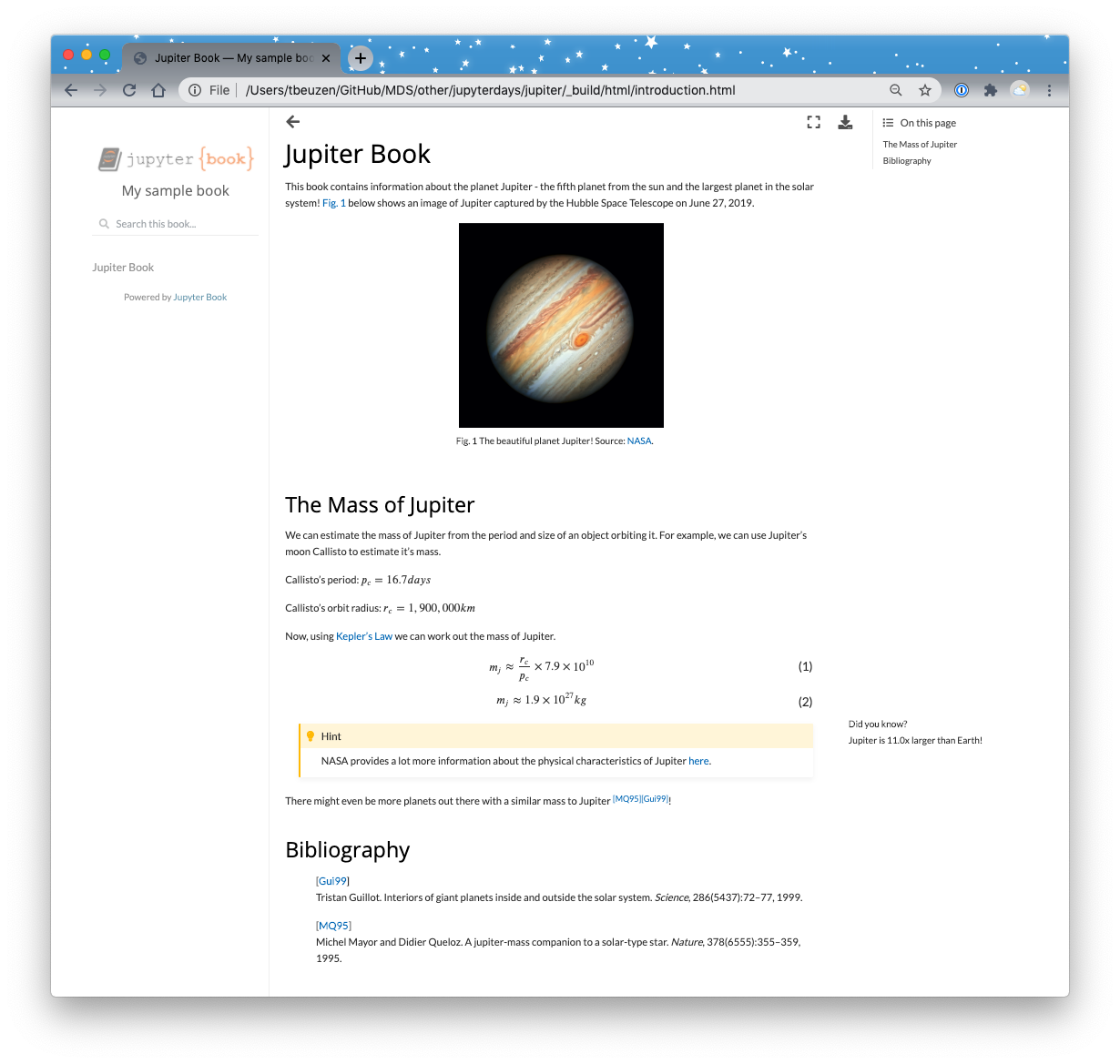
Fig. 32 The final build of the introduction page of our Jupiter book.¶

5.3. Adding a Jupyter Notebook Content File¶

In the last section we explored adding content to our book through a markdown .md file. You can also add content using a Jupyter Notebook!

All of the same formatting and style workflows we saw above apply to a Jupyter Notebook too - simply add them to a markdown cell and you’re on your way! The real utility of a Jupyter Notebook is that we can include code and code output in our book!

Let’s get started with the following:

Create a new notebook called great_red_spot.ipynb;
Add this file to your _toc.yml;
Add a markdown cell with the following content:

# The Great Red Spot

Jupiter’s iconic Great Red Spot (GRS) is actually an enormous storm that is bigger than Earth that has raged for hundreds of years! {numref}`great-red-spot` below shows an image of Jupiter captured by the Hubble Space Telescope on June 27, 2019.

```{figure} https://solarsystem.nasa.gov/system/resources/detail_files/626_PIA21775.jpg
---
height: 300px
name: great-red-spot
---
Jupiter's Great Red Spot! Source: [NASA](https://solarsystem.nasa.gov/resources/626/jupiters-great-red-spot-in-true-color/?category=planets_jupiter).
```

Jupiter's GRS has been observed to be shrinking for about the last century and a half! [Here](https://github.com/UBC-DSCI/jupyterdays/tree/master/jupyterdays/sessions/beuzen/data) is some data of the length of the GRS spanning the last ~150 years which we can use to investigate this phenomenon.

Now try building your book (jb build ./) to make sure everything is looking okay! Using the left-side content bar, navigate to the new page “The Great Red Spot” which should look like this:

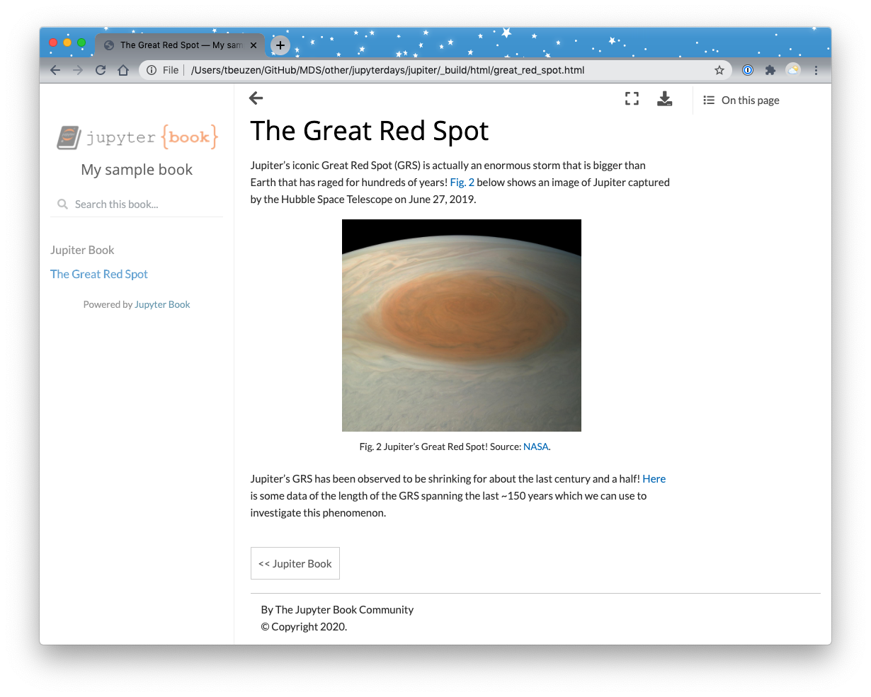
Fig. 33 The build of our new page on Jupiter’s Great Red Spot.¶

Okay great! Now let’s import that data we referenced so that we can create some plots.

Create a new code cell underneath the current markdown cell and add the following code to read in our dataset of the GRS as a Pandas Dataframe.

import pandas as pd
pd.options.plotting.backend = "plotly"

url = "https://raw.githubusercontent.com/UBC-DSCI/jupyterdays/master/jupyterdays/sessions/beuzen/data/GRS_data.csv"
df = pd.read_csv(url)
df['Year'] = df['Year'].astype(int) 
df.head()

Note

We are printing output to the display with the use of df.head() and this will show up in our rendered Jupyter Book!

If you re-build your book (jb build ./) at this point, you’ll see something like the following:

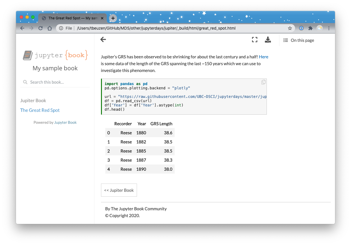
Fig. 34 A dataframe of the size of Jupiter’s Great Red Spot.¶

Now, we can use this data to create some plots.

Plots in your Jupyter Book may be static (e.g., matplotlib, seaborn) or interactive (e.g., altair, plotly, bokeh). See the official Jupyter Book documentation for more information on including plots in your Jupyter Book.

For this tutorial, we will create a few example plots using Plotly (through the Pandas backend).

Let’s first create a simple scatter plot of our data. Create a new code cell in your notebook and add the following code:

import plotly.io as pio
pio.renderers.default = "notebook"
fig = df.plot.scatter(x="Year", y="GRS Length", color="Recorder",
                      range_x=[1870, 2030], range_y=[10, 40],
                      width=650, height=400)
fig.update_layout(title={'text': "Great Red Spot Size", 'x':0.5, 'y':0.92})
fig.update_traces(marker=dict(size=7))

While we’re at it, let’s also create an animated plot. Create another new code cell and add the following code:

fig = df.plot.scatter(x="Year", y="GRS Length",
                      animation_frame="Year",
                      range_x=[1870, 2030], range_y=[10, 40],
                      width=600, height=520)
fig.update_layout(title={'text': "Great Red Spot Size Animation", 'x':0.5, 'y':0.94})
fig.layout.updatemenus[0].buttons[0].args[1]["frame"]["duration"] = 200
fig.update_traces(marker=dict(size=10))

Attention

Plotly has different renderers available to output plots. You may need to experiment with renderers to get the output you want in your Jupyter Book - I’ve found that the pio.renderers.default = "notebook" works with the current version of Jupyter Book.

Now, let’s re-build our book (jb build ./) and take a look!

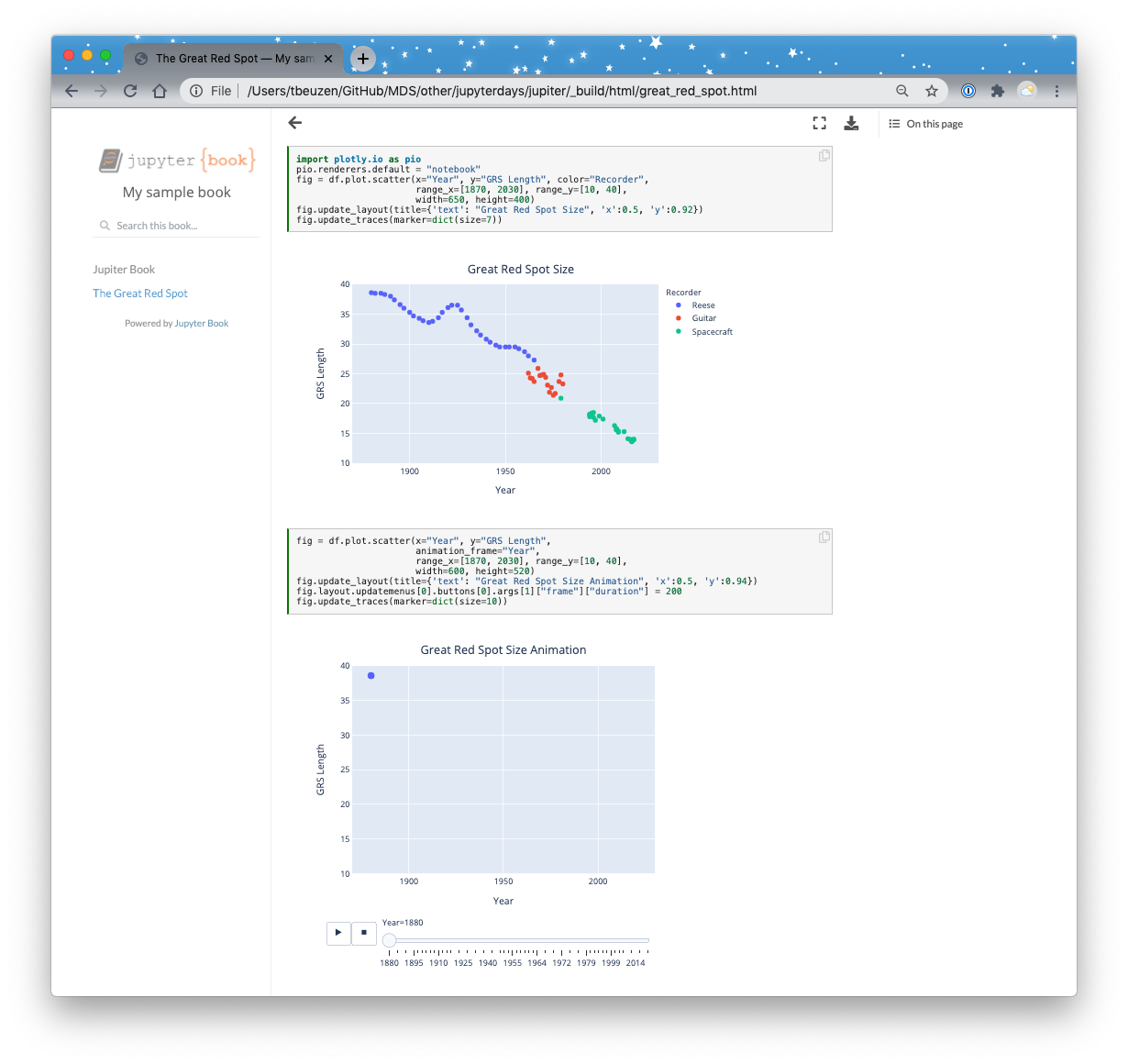
Fig. 35 Some plots of the Jupiter Great Red Spot data.¶

You may want to hide some of the code in your book - no problem! That’s easily done with Jupyter Book too. There are a few ways to hide content in your Jupyter Book as documented in the official docs.

The one we are interested in here is hiding code input. We can do that easily by adding the tag hide-input to the cell we wish to hide. There are various ways to add tags to cell in Jupyter Notebooks. In Jupyter Lab, click the gear icon in the left side-bar, and then add the desired tag as shown below:

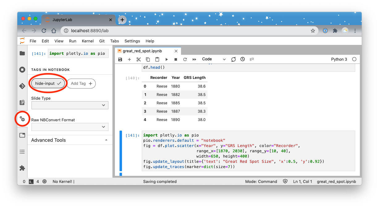
Fig. 36 Adding the “hide-content” tag to a cell in Jupyter Lab.¶

Go ahead and add the hide-input tags to both plotting cells in your great_red_spot.ipynb file. When you re-build the book, you’ll see that the code input is hidden (but can be toggled with the + icon):

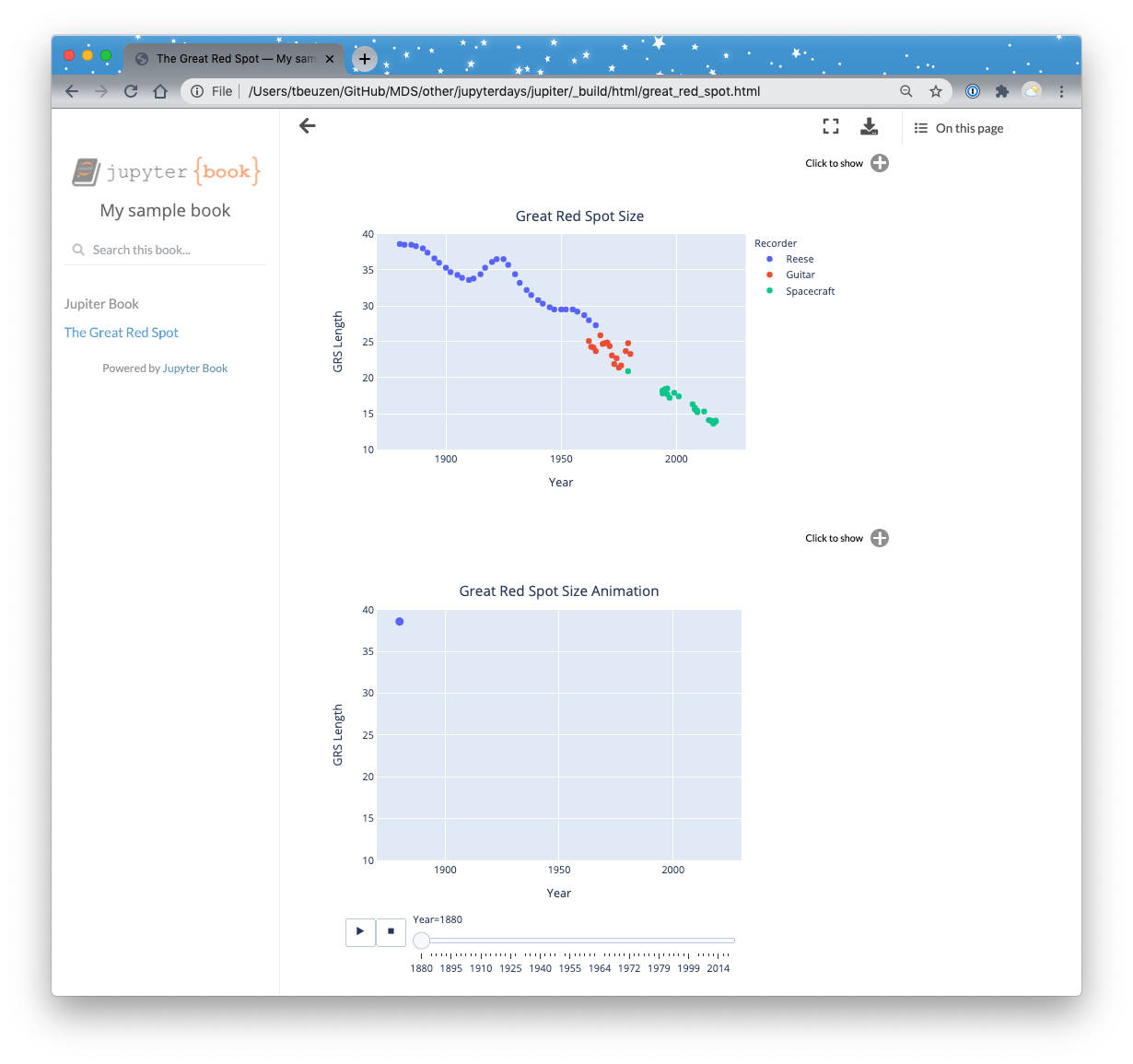
Fig. 37 Some plots of the Jupiter Great Red Spot data with the code input hidden!¶

Hint

You can also store notebook content like values, plots, or dataframes in variables that can be used throughout your notebook using the glue tool, which is described in more detail in the official Jupyter Book documentation.

6. Publishing a Book Online¶

Okay, we now have a beautiful book about Jupiter that we’d like to share with the world! The process of publishing your book online is described in the Jupyter Book documentation - which I contributed to :).

The quickest option for publishing your book online is to use GitHub Pages and you can get up and running in just a few easy steps:

Create a new GitHub repository to host your book (make your repository public and do not initialize with a README file).

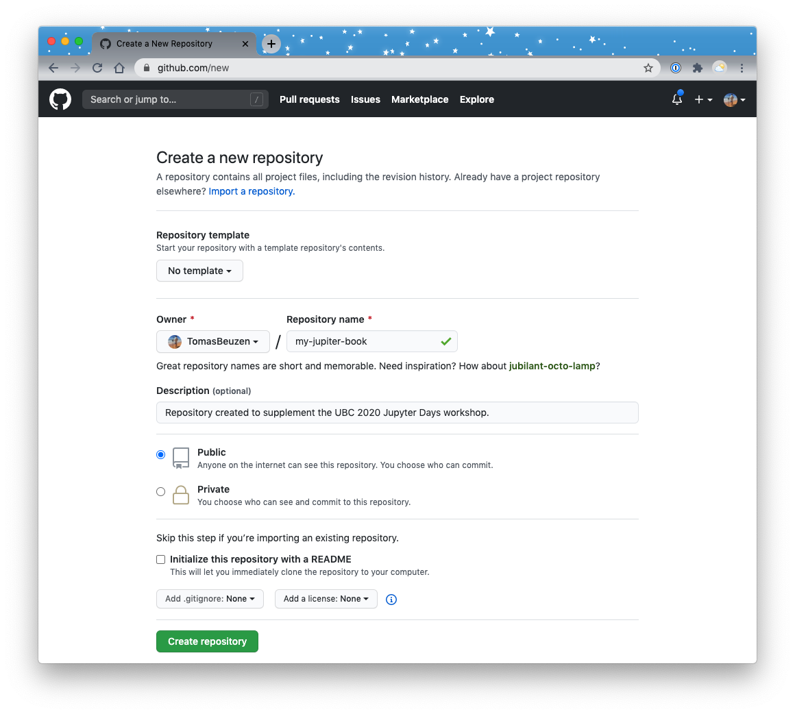
Fig. 38 Creating a new GitHub repository.¶
Navigate to your local book’s root directory from the command line and link it to your new remote GitHub repository with (GitHub provides you with instructions on how to do this):
```
git init
git remote add origin git@github.com:<user>/<repo-name>.git
git add .
git commit -m "first commit"
git push -u origin master
```
Install the ghp-import tool:
```
pip install ghp-import
```
From your book’s local root directory (which should contain the _build/html folder) call ghp-import and point it to your HTML files, like so:
```
ghp-import -n -p -f ./_build/html
```

Note

ghp-import works by copying all of the contents of your built book (i.e., the _build/html folder) to a branch of your repository called gh-pages, and pushes it to GitHub.

After a few minutes your site should be viewable online at a url such as: https://<user>.github.io/<myonlinebook>/. For example, my repository is available at: http://www.tomasbeuzen.com/my-jupiter-book/introduction.html

Attention

My GitHub is configured to publish pages using my personal domain <www.tomasbeuzen.com>. The default domain is tomasbeuzen.github.io and your link will have a similar syntax, unless otherwise configured.

You can also choose to automate the build and deploy process with GitHub Actions - for example, every time you push new content to your GitHub repository, your book can be automatically built and deployed. Implementing this automatic deployment is described here.

Note

For those interested, I’m in the process of cleaning up a cookiecutter template for making Jupyter Books that includes the GitHub Actions workflow files.

7. Interactive Content¶

Last but not least - let’s add interactivity to our book. Because Jupyter Books can be built with Jupyter Notebooks, you can enable users to launch live Jupyter sessions in the cloud directly from your book and interact with your code content. Jupyter Book currently facilitates interactivity through Binder, JupyterHub, Google Colab and ThebeLab.

7.1 Binder¶

If your Jupyter Book is hosted online on GitHub, you can automatically insert buttons in your Jupyter Book that link to its Jupyter Notebooks running in Binder. When a user clicks the button, they’ll be taken to a live version of the page. Assuming your code doesn’t require a significant amount of CPU or RAM, you can use the free, public BinderHub running at https://mybinder.org.

To set up Binder link buttons in each page of your Jupyter Book, add the following configuration to your _config.yml file:

launch_buttons:
  binderhub_url: "https://mybinder.org"  # The URL for your BinderHub (e.g., https://mybinder.org)

repository:
  url          : https://github.com/TomasBeuzen/my-jupiter-book  # The URL to your book's repository
  path_to_book : ""  # A path to your book's folder, relative to the repository root.
  branch       : master  # Which branch of the repository should be used when creating links

We’ll also need to add a .binder/requirements.txt file to help build our interactive Binder environment. In your book’s root directory, create, a new text file .binder/requirements.txt:

mkdir .binder
touch .binder/requirements.txt

Add the following content to that file (which points to the existing requirements.txt file in our book’s root):

-r ../requirements.txt

In the requirement.txt file in our book’s root directory, change the content to:

jupyter-book
ghp-import
sphinx-thebe
pandas
plotly

Note

The jupyter-book and ghp-import package are not actually required here but they are required for automating the building of your book with GitHub Actions so I’ve left them in.

Re-build your book (jb build ./) and open up the “The Great Red Spot” page and you’ll see a new rocket ship button at the top of the screen that allows you to launch your notebook in Binder!

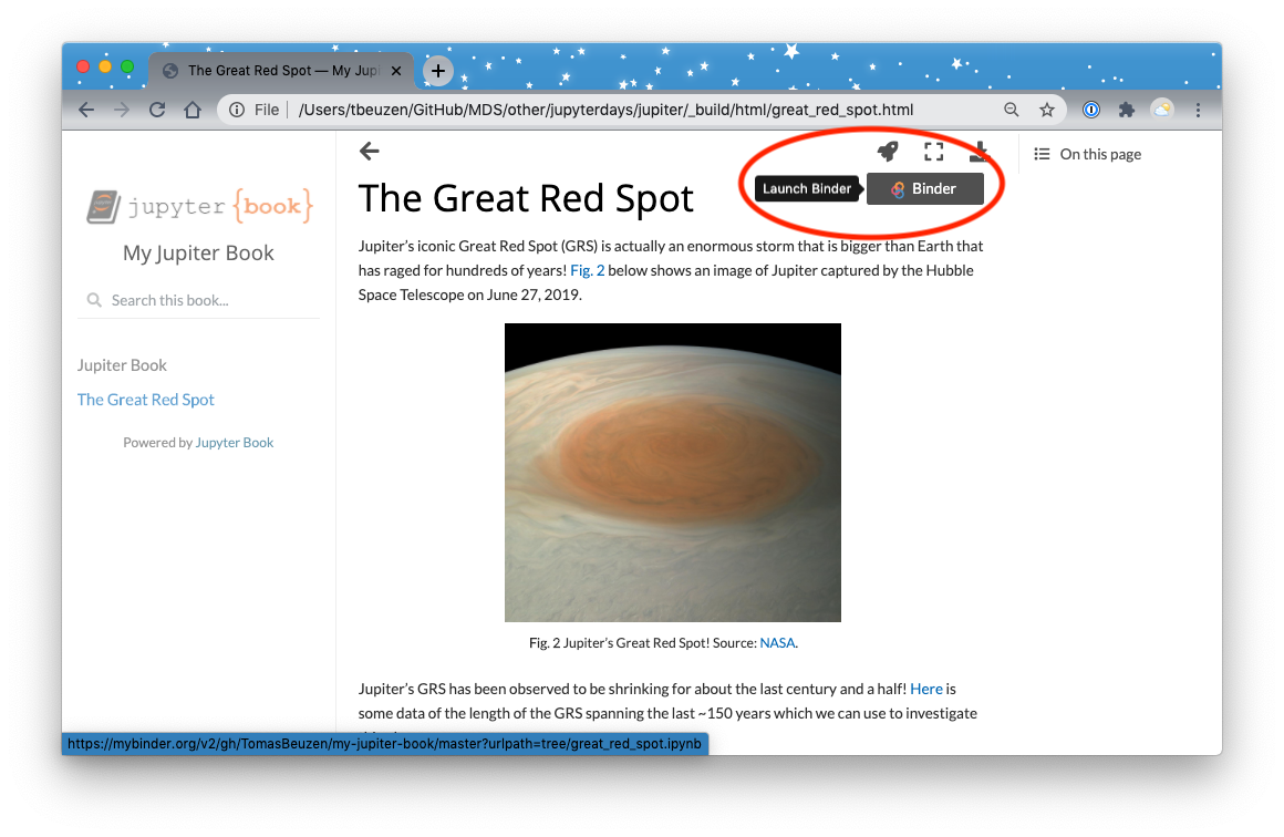
Fig. 39 Adding interactivity through Binder.¶

7.2 ThebeLab¶

Thebe Lab is a tool that turns your static HTML pages interactive, powered by a kernel. It is a work-in-progress which you can follow in the official docs. This functionality allows users to run code and see outputs in your Jupyter book without leaving the page!

To set up Thebelab in your Jupyter Book, add the following configuration to your _config.yml file:

launch_buttons:
  notebook_interface : "classic" # The interface interactive links will activate ["classic", "jupyterlab"]
  binderhub_url      : "https://mybinder.org"
  thebe              : true

repository:
  url          : https://github.com/TomasBeuzen/my-jupiter-book  # The URL to your book's repository
  path_to_book : ""  # A path to your book's folder, relative to the repository root.
  branch       : master  # Which branch of the repository should be used when creating links

sphinx:
  extra_extensions:
    - sphinx_thebe

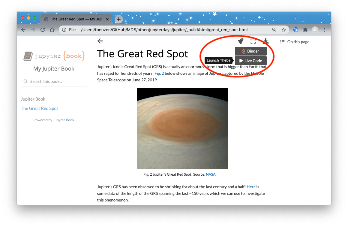
Fig. 40 Adding interactivity through ThebeLab.¶

You can have code cells (even hidden ones) execute automatically when Thebe is initialized! Read more about that here.

8. Wrapping Up¶

Congratulations! You’ve made it to the end of the tutorial. I hope you learned something about how useful Jupyter Book could be in creating and distributing open-source material (and maybe you learned something about the planet Jupiter too!).

I’ll leave you with a few examples of Jupyter Book being used out in the wild:

UBC JupyterDays 2020

Jupyter Book¶

1. Introduction¶

I’m Tom. Nice to meet you!¶

1.1. Jupyter Book¶

1.2. Key Jupyter Book Features¶

1.3 Key Jupyter Book Information¶

2. Jupyter Book Tutorial¶

3. Installing Jupyter Book¶

4. Creating a Book Structure¶

5. Adding Content¶

5.1. Re-structuring Our Book Directory¶

5.2. Adding a Markdown Content File¶

5.2.1. Markdown Text¶

5.2.2. Figures¶

5.2.3. Math and Equations¶

5.2.4. Controlling the Page Layout¶

5.2.5. Admonitions¶

5.2.6. Citations and a Bibliography¶

5.3. Adding a Jupyter Notebook Content File¶

6. Publishing a Book Online¶

7. Interactive Content¶

7.1 Binder¶

7.2 ThebeLab¶

8. Wrapping Up¶