Interactive exploration with widgets and dashboards
Here, we will use a motivating example that looks at atmospheric CO\(_2\) data measured at Mauna Loa. We will be using:
Jupyter Widgets to connect interactive controls (sliders, toggle buttons, etc) to code and
Voilà dashboards to create computational “apps”
The example we follow is adapted from the Intro-Jupyter tutorial from ICESat-2Hackweek, which has contributions from: Shane Grigsby (@espg), Lindsey Heagy (@lheagy), Yara Mohajerani (@yaramohajerani), and Fernando Pérez (@fperez).
1. 👋 Hello

Fig. 50 Hi, I’m Lindsey
I am currently a Postdoc at UC Berkeley in the Department of Statistics
I will be joining UBC-EOAS as an Asst. Prof in July 2021
My PhD was in computational geophysics (modelling and inversions)
Throughout my academic career, I have been involved in development of open source software in Python & open educational resources
2. Motivating example: CO\(_2\) at Mauna Loa
Question: Based on historical CO\(_2\) data, can we estimate what CO\(_2\) concentrations will be in the future?
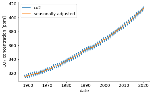
Scripps institute of Oceanography has a research station at Mauna Loa in Hawaii where they have been measuring atmospheric CO\(_2\) since 1958. The data we will focus on are the seasonally adjusted data.
Data Source
C. D. Keeling, S. C. Piper, R. B. Bacastow, M. Wahlen, T. P. Whorf, M. Heimann, and H. A. Meijer, Exchanges of atmospheric CO2 and 13CO2 with the terrestrial biosphere and oceans from 1978 to 2000. I. Global aspects, SIO Reference Series, No. 01-06, Scripps Institution of Oceanography, San Diego, 88 pages, 2001. https://scrippsco2.ucsd.edu/data/atmospheric_co2/primary_mlo_co2_record.html
import matplotlib.pyplot as plt
import numpy as np
import pandas as pd
from matplotlib import rcParams
rcParams["font.size"] = 14
2.1 What are our data?
Before we dive into widgets, lets take a look at our data. The measured atmospheric data are the column titled co2. In this data set, there is one measurement per month. The seasonally adjusted data are what we will work with – these smooth over the 6 month seasonal variations. For details on how this correction is applied, see the original excel file.
co2_data_source = "./data/monthly_in_situ_co2_mlo.csv"
co2_data = pd.read_csv(
    co2_data_source, skiprows=np.arange(0, 56), na_values="-99.99"
)

co2_data.columns = [
    "year", "month", "date (int)", "date", "co2", "seasonally adjusted",
    "fit", "seasonally adjusted fit", "co2 filled", "seasonally adjusted filled"
]
fig, ax = plt.subplots(1, 1, figsize=(8, 5))
co2_data.plot("date", ["co2", "seasonally adjusted"], ax=ax)
ax.set_ylabel("CO$_2$ concentration [ppm]")
Text(0, 0.5, 'CO$_2$ concentration [ppm]')
In the demo repository, we will explore building linear models using the “eye-ball” norm with widgets. To follow along:
UBC Students & Faculty:
or if you don’t have a UBC CWL:

or you can follow the installation instructions on the repository
3. Jupyter widgets
Jupyter widgets allow you to connect interactive controls such as slide bars and toggle buttons to your code.
They can be used to create “notebook apps” that abstract away details of the code and focus conversations on the role of parameters in a computation, or be a quick way to create a “Just-in-time-research-GUI” (GUI: graphical user interface) to explore results.
Getting started
Widgets can be installed with pip
pip install ipywidgets
jupyter nbextension enable --py widgetsnbextension
or conda (which also enables the extension)
conda install -c conda-forge ipywidgets
To enable the Jupyter Lab extension
jupyter labextension install @jupyter-widgets/jupyterlab-manager
For your first interaction with widgets, I recommend trying out interact. The interact function ipywidgets.interact is a quick way to create user interface controls on your functions. At the most basic level, interact autogenerates controls for function arguments, and then calls the function with those arguments when you manipulate the controls interactively. To use interact, you need to define a function that you want to explore.
Demo!
The ubc-jupyterdays-2020-widgets contains notebooks which demonstrate using widgets to explore data as well as a notebook which covers some of the basics of using widgets.
UBC Students & Faculty can run on the UBC Syzygy:
or if you don’t have a UBC CWL you can use:
4. Voilà Dashboards
Voilà turns Jupyter notebooks into standalone web applications.
Unlike the usual HTML-converted notebooks, each user connecting to the Voilà tornado application gets a dedicated Jupyter kernel which can execute the callbacks to changes in Jupyter interactive widgets.
The intro blog provides an overview and resources for getting up and running with Voilà
The Voilà gallery has a collection of examples built with Voilà and Jupyter widgets.
Getting Started
Voilà can be installed using conda
conda install -c conda-forge voila
or from PyPI
pip install voila
Once Voilà has been installed,
you can run it as a standalone server
voila notebook.ipynb
or as a server extention by changing the url to
<url-of-my-server>/voila(e.g. if you launchedjupyter lablocally, and it was running athttp://localhost:8888/lab, then then Voilà would be accessed athttp://localhost:8888/voila.there is also a JupyterLab extention for previewing your dashboard
jupyter labextension install @jupyter-voila/jupyterlab-preview
by default, Voilà will strip out the source code from view. It can be displayed if the option
strip_sourcesis set to False
Demo!
![]()