Introduction to JupyterLab¶

Introduction¶

I am a PhD student in Biomedical Engineering at the University of Toronto, where I use computational and experimental approaches to better understand fundamental stem cell decisions. I am excited to be starting as a Post-Doc for the UBC Master of datascience program this fall!

Learning outcomes¶

After this seminar you will be able to

Launch JupyterLab via the syzygy cloud platform
Use the Notebook interface inside Jupyterlab
Know your way around the JupyterLab user interface

Outline¶

What is JupyterLab
How to access JupyterLab using a web browser
Using Jupyter Notebooks
- Working with text via Markdown cells
- Interactive figure creation
- Static figure creation
- Exporting notebooks
The JupyterLab sidebar
Additional JupyterLab applications
- How to get help in the notebook

What is JupyterLab¶

The most rudimentary interaction with programming languages such as R and Python is via interactive shells run from a terminal.
- This provides access to the full functionality of the language, but is a barebones experience without any conveniences added.
- If you want to edit a script or view a plot that you created, you need to open a text editor and image viewer separately.
If you prefer a more holistic experience, with many of conveniences nicely organized in the same interface, you can use an integrated development environment (or IDE for short).
- IDEs often include a shell, a file browser, debugging tools, a text editor with autocompletion and syntax highlighting, and an area where plots show up.
- A core idea of IDEs is to provide all the tools you need in one place, and we will see later today how it is also possible to things like version control from within your IDE.
- Commons IDEs that you might have heard of include Visual Studio Code and RStudio, and today we will be learning about JupyterLab, which is and IDE to work with many programming languages, including R, Python, Julia, and many more.
  - A core concept tightly linked to JupyterLab are Jupyter Notebooks, which will be one of the main topics in this talk, but first, let’s see how we can launch JupyterLab.

How to access JupyterLab using a web browser¶

We could install and run JupyterLab just like any other program on Windows, MacOS, or Linux.
However, one of the advantages of JupyterLab is that it is easy to use without installing anything, which is really handy when teaching.
To try JupyterLab, use your web browser to visit the following address https://ubc.syzygy.ca/ and login with your CWL (Firefox, Chrome, and Safari are supported)
- If you don’t have UBC CWL, you can instead use this address https://pims.syzygy.ca/ and login with a Google account.
  - The PIMS version lets you explore the JupyterLab interface, but does not include all the extensions and package we will cover in this workdshop.
syzygy.ca is a project of the Pacific Institute for the Mathematical Sciences, Compute Canada and Cybera to bring JupyterLab to researchers, educators and innovators across Canada.
- The name is an astronomical term referring to the alignment of celestial objects, and here it is used to represent the alignment of text, math, and code inside Jupyter notebooks.
Thanks to that JupyterLab is built entirely using web technologies,
it can be rendered in a browser without the need to install anything,
- The necessary packa TDOO
The reason we can use
Once you log in, a server will be started for you somewhere in the cloud, e.g. at compute Canada.
Once logged in, you will see list of files, this is the traditional interface for working with Jupyter Notebooks, and to instead access JupyterLab, you can change the part of the URL after the final forward slash that says tree? to lab.
- True to its name, and as a tribute to Galileo Galilei the loading animation illustrates the planet Jupiter orbited by three of the moons Gallelei identified.
its interface is built largely using Javascript and Typescript, which means all that nee

Using Jupyter Notebooks¶

We’re greeted by the launcher tab where we see that we can start either a Notebook or Console for Python or R, as well as some other utility programs.
Let’s start by explaining one of the most popular options, the Jupyter Notebook.
The Notebook provides and interface where you can mix text, code, mathematical expressions, plot output, videos, and more, all in the same file.
- So instead of the traditional IDE experience where you would write code in a text file and then have figures pop up in a different panel, this information now all resides in the same document, which facilitates reproducibility and collaboration.
- The Notebooks can be exported to many formats, including PDF and HTML, which makes it easy to share your project with anyone.

The cell that is encircled in blue is where we can input Python code, click here and type any mathematical expression, and then run the cell by clicking the play button in the top toolbar:

3 + 4

As you can see, the output is returned just under input, and a new input cell was created.
- We could also have clicked the plus sign to create a new cell.
Here, we can do anything we can do in Python, e.g. variable assignment:

a = 5

There is no output because we just assigned a value to a variable, without asking for the value of that variable, which we can do by typing out the variable name:

Jupyter Notebooks also supports editing code on multiple lines, so we could have done this instead:

a = 3
a

You might have noticed that there is a little counter on the left of each cell. This counter keeps track of in which order the cells were executed, so that you are aware if cells have been run out of sequential order.
The counter symbol changes to an * when a computation is running, to indicate that Python is busy and won’t be able to execute new cells until the current one finishes (the delay is only noticeable for longer computations).
We can also click this blue bar to the left to collapse and expand the output and input.
- This can be handy if we have a long code cell, or some notes that we’re planning on moving later.
The notebook is saved automatically every two minutes, and it can be saved manually by clicking the floppy disk symbol in the toolbar, or by hitting Ctrl + s. Both input and output cells are saved, so any plots that you make will be present in the notebook next time you open it, without needing to rerun the code cells.
Other important icons in the toolbar are the ones to cut, copy, and paste a cell.
- If you want to get rid of a cell, you can cut it out without pasting in back in.
The remaining icons are:
- the play button to run a cell (which we already used),
- the stop button which we can use if a cells has gotten stuck running some code and we want to interrupt it,
- the restart button which restarts the background Python process that is connected to the notebook (so if we click this, our variables will need to be redefined),
- and last the restart and run all button (this is really important and should always be executed before sharing a notebook, to make sure that everything will work when someone else runs it from top to bottom, since the cells can be executed out of order)
You can also access these by right clicking on a cell.

Working with text via Markdown cells¶

You can change the input cell type from Python code to Markdown by clicking on the little dropdown menu in the toolbar that reads “Code”.

Markdown is a simple formatting system which allows you to document your analysis within the notebook. This is also great for creating tutorials and even books as we will see later.
It is a plain text format that includes brief markup tags that indicates how text should be rendered, e.g. * indicates italics and ** indicates bold typeface. If you have commented on online forums or used a chat application, you might already be familiar with markdown. Below is a short example of the syntax:

### Heading level three

- A bullet point
- *Emphasis in italics*
- **Strong emphasis in bold**
- This is a [link to learn more about markdown](https://guides.github.com/features/mastering-markdown/).
- Support for $\LaTeX$ equations: 
$$f'(a) = \lim_{x \to a} \frac{f(x) - f(a)}{x-a}$$

will be rendered as:

Heading level three¶

A bullet point
Emphasis in italics
Strong emphasis in bold
This is a link to learn more about markdown.
Support for $\LaTeX$ equations: $$f'(a) = \lim_{x \to a} \frac{f(x) - f(a)}{x-a}$$

Let’s create a cell with a heading for this tutorial # JupyterLab tutorial, and then click and drag to position it on the top of the notebook.

Static figure creation¶

To show an example of how plots are rendered, we will use the seaborn plotting package which is a high level interface to the more widely known matplotlib package.
This is just to illustrate how plots show up in the notebook rather than a tutorial on how to plot in Python so I will not go into details on what these commands mean.

import seaborn as sns

# Load the example mpg dataset
mpg = sns.load_dataset("mpg")
# Plot miles per gallon against horsepower
sns.relplot(x="horsepower", y="mpg", hue="origin", size="weight",
            sizes=(40, 400), alpha=0.4, data=mpg)

<seaborn.axisgrid.FacetGrid at 0x7f25e7e7ca50>

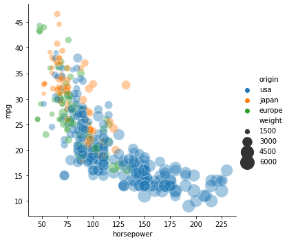
The above is a static figure, which means an image is created and included in the notebook.
- To save this image, you can either use a save command in the plotting library or you can hold shift and right click. Just right clicking is the JupyterLab menu, but holding shift brings up the browser menu, which includes the common options for images such as open in new tab and save.

Interactive figure creation¶

Plotting libraries that create interactive figures using HTML and Javascript can also be used inside notebooks.
Below is a more complex example just to show the extent of what is possible.
- Again, no need to worry about the specific syntax here, the takeaway is that interactivity via animation, mouse hover, zooming, and more is possible inside notebooks.
- This could be extended by using widgets to build dashboards inside Notebooks, which we will talk more about during the third day of the workshop.

import plotly.express as px

gm = px.data.gapminder()
px.scatter(
    gm, 'gdpPercap', 'lifeExp', color='continent', size='pop',
    hover_name='country', hover_data=['year'], animation_frame='year',
    size_max=45, log_x=True, range_x=[100, 100_000], range_y=[25, 90])

Exporting notebooks¶

The combination of code, plots, and markdown is powerful. With these three elements, you can keep all your analysis code and interpretations in the same document, instead of spread across different files.
Notebooks are excellent tools to build entire reports, since they can contain formatting such as a table of contents, links to sections and files, footnotes, images, bibliographies, and even videos, which we will learn more about later in the workshop.
You can export the notebook to different file types via File –> Export Notebook As…. (When you export to PDF for the first time on your own machine, you might be asked to download the Latex packages, which are needed to create the PDF.)
- If we would export this notebook the HTML, we would still retain the interactivity of the plots we created!

The JupyterLab sidebar¶

Now that you know the basics of how to work inside Jupyter Notebooks, let’s continue explorer the JupyterLab user interface.
The puzzle piece at the bottom is where you can install extensions.
- syzygy already comes with a several helpful extensions installed, including the ToC icon, which creates the next icon in the sidebar.
The ToC can be used to navigate between the markdown headings we have created.
- This ToC will not be included when exporting, but there are other ways to achieve that.
- You can number and even preview the code in each heading.
The next icon just shows the tabs, same as what you see on top.
The next icon is a bit more advanced as it allows you to add metadata to cells.
- One aspect worth highlighting here is the ability to denote cells as part of a slide show, that you can download via File -> Export notebook as.
The commands section is really helpful if you can’t remember a shortcut or where your command is in the menu.
- It also shows the keyboard shortcuts for each command.
The stop sign icon shows an overview of all running applications.
The topmost icon in the sidebar to the left shows the file tree of your current folder, highlights include:
- the icon for uploading files from your computer to the syzygy server
- right clicking a file to download it to your computer
- clicking the + sign takes us back to the launcher menu where we started

Additional JupyterLab applications¶

JupyterLab can run applications other than notebooks, e.g. there is a Python console, a text editor, and a terminal emulator.
- These can be opened via the launcher page or File –> New.
- Applications can be placed side by side by dragging and dropping their windows, so we could be running a terminal and notebook next to each other.

How to get help in the notebook¶

One application that is especially helpful to run next to a notebook is the Contextual Help.
This application displays documentation automatically as you type.
When you’re using unfamiliar packages and functions, it is a good habit to leave the Contextual Help open next to the notebook.
If you don’t like having a split screen, you can instead press Shift + Tab to bring up a help dialogue.
JupyterLab also supports tab completion, you can start typing a name and then press tab to see suggestions to expand to.
Additional help is available via the “Help” menu, which links to useful online resources (for example Help --> JupyterLab Reference).
If you need to restart the server, you can go to File -> Hub control panel -> Stop my server and then click Start my server -> Launch server.
- All your files will be saved between restarts, but any Python packages you have installed yourself will be reset, so you need to contact UBC IT to have additional Python packages installed with persistence.

UBC JupyterDays 2020